
In modern mechanical engineering, the design and manufacturing of spiral bevel gears represent a critical challenge due to their complex geometry and demanding performance requirements. Spiral bevel gears are widely utilized in high-power transmission systems, such as those found in automotive, aerospace, and mining equipment, owing to their superior characteristics like high overlap ratio, smooth operation, and substantial load-bearing capacity. However, the intricate nature of spiral bevel gears—encompassing their tooth geometry, meshing behavior, and sensitivity to manufacturing adjustments—makes traditional design and production processes time-consuming and costly. Typically, achieving optimal contact patterns on spiral bevel gears requires multiple physical trial cuts and machine adjustments, which rely heavily on operator expertise. To address these issues, I have developed a comprehensive virtual simulation method that replicates the actual cutting process of spiral bevel gears, specifically focusing on the Gleason system. This approach enables the generation of accurate three-dimensional models through mathematical modeling of the cutting kinematics, facilitating virtual trial cuts, parameter optimization, and enhanced contact analysis. By leveraging this methodology, manufacturers can significantly reduce costs, improve efficiency, and achieve more reliable gear performance without physical prototyping. Throughout this article, the term “spiral bevel gears” will be emphasized to underscore the centrality of these components in advanced gear systems.
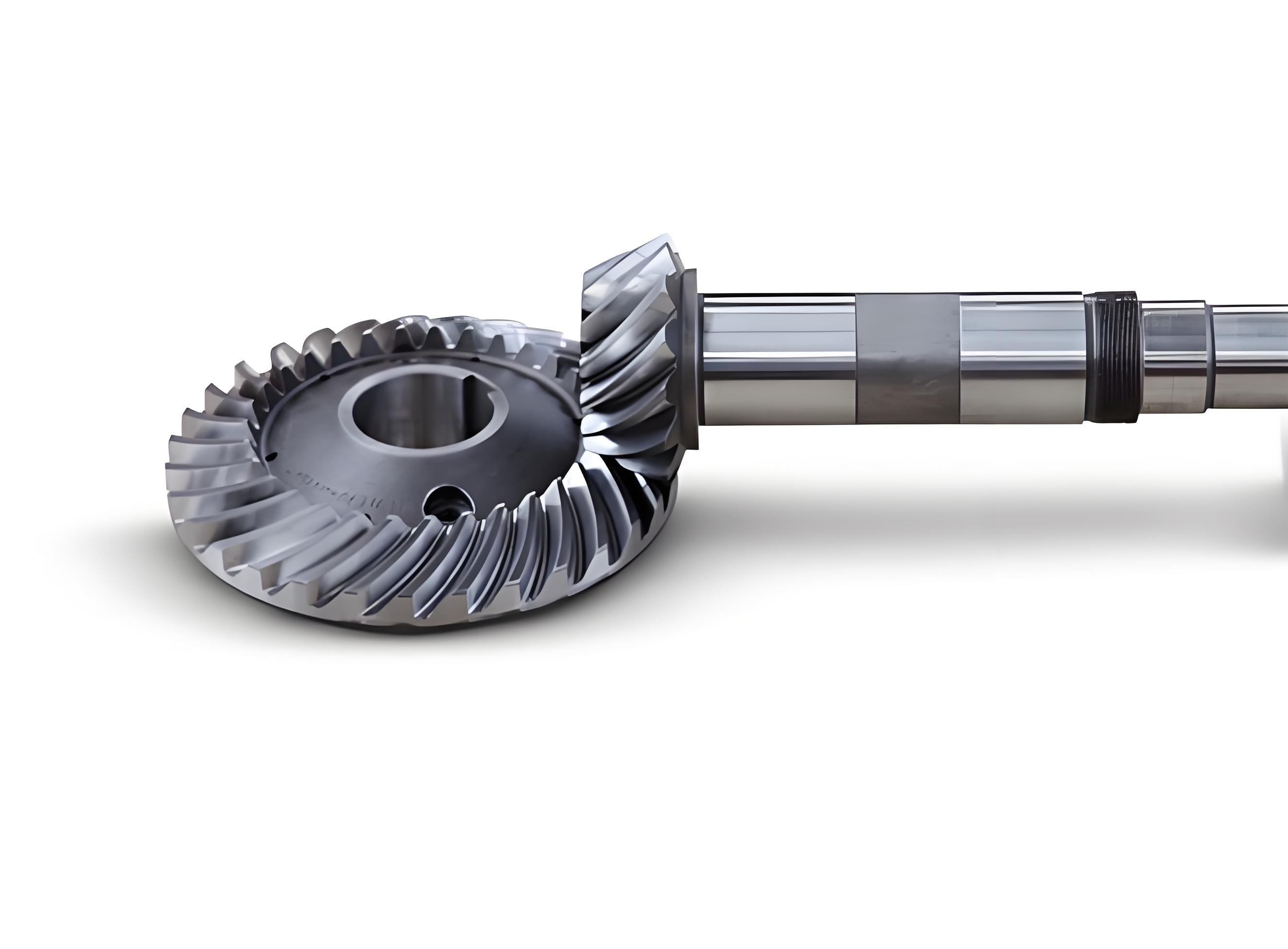
The core of this work lies in simulating the actual tooth-cutting process for spiral bevel gears, which involves modeling the interactions between the cutting tool, machine components, and gear blank. Spiral bevel gears are produced using specialized machines like the Gleason hypoid generator, where a rotating cutter head (containing multiple blades) generates the tooth surface through a relative motion with the gear blank. This process mimics the meshing of a hypothetical generating gear (or “crown gear”) with the workpiece. To accurately capture this, I established a detailed kinematic model of the Gleason machine, defining multiple coordinate systems that represent the positions and orientations of key components: the machine base, cradle, cutter head, and gear blank. These coordinate systems are essential for transforming tool paths into gear tooth coordinates, enabling precise calculation of tooth surface points. The transformation matrices between these systems incorporate various adjustment parameters—such as cradle angle, tool tilt, and workpiece offset—that influence the final geometry of spiral bevel gears. By manipulating these parameters digitally, I can simulate different machine settings and observe their effects on tooth profiles, thereby optimizing the manufacturing process for spiral bevel gears without physical trials.
To elucidate the coordinate system setup, consider the Gleason machine as comprising four main parts: the tool (cutter blade), cutter head, cradle, and workpiece. A global static coordinate system, denoted as Σ₀ (O₀X₀Y₀Z₀), is fixed at the machine center, with the Z₀-axis perpendicular to the cradle face. Additional coordinate systems are attached to moving components: Σ₁ (O₁X₁Y₁Z₁) rotates with the cradle, Σ₂ (O₂X₂Y₂Z₂) is fixed to the cutter head, Σ₃ (O₃X₃Y₃Z₃) accounts for tool inclination, and Σ₄ (O₄X₄Y₄Z₄) is rigidly attached to the cutter blade. The workpiece coordinate system, Σ₁′ (O₁′X₁′Y₁′Z₁′), is defined relative to the gear blank, with its origin at the calculation point. Transformations between these systems involve rotations and translations based on machine adjustments. For instance, the transformation from Σ₄ to Σ₀ is given by a homogeneous matrix M₄₀, which depends on cradle rotation angle q, tool rotation angle θ, and other parameters. Similarly, the transformation from Σ₀ to Σ₁′ involves offsets like vertical wheel setting E, axial wheel setting X, and bed setting X_B, along with workpiece rotation. The composite matrix M₄₁′ = M₄₀ * M₀₁′ maps cutter coordinates to workpiece coordinates, facilitating the derivation of tooth surface points. This mathematical framework is foundational for simulating the cutting of spiral bevel gears, as it encapsulates the dynamic interactions during gear generation.
The cutting process for spiral bevel gears is mathematically modeled by representing the cutter blade as a line in the tool coordinate system and tracking its motion relative to the gear blank. Each blade on the cutter head has a cutting edge described by a parametric equation in Σ₄. For a single blade at time t, the edge can be expressed as a line in the X₄O₄Z₄ plane, with parameters accounting for blade geometry. Assuming a straight cutting edge, the equation is:
$$ \begin{cases} X_4 = r_a u + r_a \\ Y_4 = 0 \\ Z_4 = -r_a u \cot \alpha \end{cases} $$
where \( u \) is a parameter, \( r_a \) is the cutter tip radius, and \( \alpha \) is the pressure angle of the blade. This equation defines the position of the cutting edge in the tool system. Since the cutter head contains multiple blades spaced evenly around its axis, the equation for any blade can be derived by applying a rotation transformation about the Z₄-axis. For example, the second blade, offset by an angle \( 2\pi/n \) (where n is the number of blades), has coordinates:
$$ \begin{cases} X_4 = r_a \cos(2\pi/n) u + r_a \cos(2\pi/n) \\ Y_4 = r_a \sin(2\pi/n) u + r_a \sin(2\pi/n) \\ Z_4 = -r_a \sin(2\pi/n) u \end{cases} $$
These equations are transformed into the workpiece coordinate system Σ₁′ using the matrix M₄₁′, which varies with time due to the rotations of the cradle, cutter head, and workpiece. Let T_t = M_{Δt}^{tool} * M₄₁′(t) represent the combined transformation at time t, where M_{Δt}^{tool} accounts for cutter head rotation over a small time increment Δt. The cutting edge in Σ₁′ becomes a parametric line, and as the machine operates, successive blades intersect the gear blank, generating a series of “cut marks” that collectively form the tooth surface of spiral bevel gears. To compute points on this surface, I analyze the intersections between cut marks from adjacent blades at different times, ensuring accuracy even when the lines are skew in space. This approach mimics the actual material removal process, crucial for realistic modeling of spiral bevel gears.
Deriving explicit equations for tooth surface points requires solving for intersections between lines representing cut marks. Consider two consecutive cuts: at time t, the first blade leaves a line L₁ in Σ₁′, and at time t+Δt, the second blade leaves a line L₂. Using the transformation matrices, these lines are expressed parametrically. If L₁ and L₂ intersect, the intersection point p is computed directly; if they are skew lines (non-intersecting and non-parallel), point p is taken as the midpoint of the shortest segment between them (the common perpendicular). This ensures a continuous tooth surface for spiral bevel gears. The coordinates of point p in Σ₁′ are derived from the line equations and transformation parameters. For instance, when lines intersect, the coordinates (X_p, Y_p, Z_p) are given by:
$$ X_p = r_a t_{11} \cos(\omega_1 \Delta t) + r_a t_{12} \sin(\omega_1 \Delta t) – a \left\{ \left[ (r_a t_{11} \cos(\omega_1 \Delta t) + r_a t_{12} \sin(\omega_1 \Delta t) – r_a \cos(2\pi/n) t_{11}(\Delta t) + r_a \sin(2\pi/n) t_{12}(\Delta t) \right] c’ + a’ \left[ r_a \cos(2\pi/n) t_{13}(\Delta t) + r_a \sin(2\pi/n) t_{23}(\Delta t) \right] \right\} / (a c’ – a’ c) $$
$$ Y_p = r_a t_{12} \cos(\omega_1 \Delta t) + r_a t_{11} \sin(\omega_1 \Delta t) – b \left\{ \left[ (r_a t_{11} \cos(\omega_1 \Delta t) + r_a t_{12} \sin(\omega_1 \Delta t) – r_a \cos(2\pi/n) t_{11}(\Delta t) + r_a \sin(2\pi/n) t_{12}(\Delta t) \right] c’ + a’ \left[ r_a \cos(2\pi/n) t_{13}(\Delta t) + r_a \sin(2\pi/n) t_{23}(\Delta t) \right] \right\} / (a c’ – a’ c) $$
$$ Z_p = r_a t_{13} + c \left\{ \left[ (r_a t_{11} \cos(\omega_1 \Delta t) + r_a t_{12} \sin(\omega_1 \Delta t) – r_a \cos(2\pi/n) t_{11}(\Delta t) + r_a \sin(2\pi/n) t_{12}(\Delta t) \right] c’ + a’ \left[ r_a \cos(2\pi/n) t_{13}(\Delta t) + r_a \sin(2\pi/n) t_{23}(\Delta t) \right] \right\} / (a c’ – a’ c) $$
where \( a, b, c, a’, b’, c’ \) are coefficients derived from transformation matrix elements, and \( \omega_1, \omega_2, \omega_3 \) are angular velocities of the workpiece, cradle, and cutter head, respectively. By iterating this process for multiple blades and time steps, a dense point cloud representing the tooth surface of spiral bevel gears is generated. These points serve as the basis for three-dimensional reconstruction, enabling the creation of accurate CAD models that reflect actual cutting conditions. The ability to compute these points dynamically allows for virtual adjustment of machine parameters, facilitating optimization of spiral bevel gears for improved contact patterns and performance.
To validate the methodology, I implemented the algorithms in a programming environment (using Visual Basic) and applied them to a specific case study of spiral bevel gears. The gear parameters were set according to Gleason standards: 11 teeth, module of 9, and standard pressure angle. The simulation involved computing tooth surface points by modeling the relative motions as described. The point cloud was then exported to CAD software (e.g., Pro/ENGINEER) for surface reconstruction. Using reverse engineering techniques, points were fitted into curves, which were then lofted to form surfaces, ultimately yielding a solid 3D model of the spiral bevel gear. This process demonstrated the feasibility of virtual cutting for spiral bevel gears, as the model accurately captured tooth geometry, including curvatures and offsets inherent to the Gleason system. The table below summarizes key parameters used in the simulation for spiral bevel gears:
| Parameter | Symbol | Value | Description |
|---|---|---|---|
| Number of Teeth | z | 11 | Teeth count on the gear |
| Module | m | 9 mm | Module at the gear end face |
| Cutter Tip Radius | r_a | 150 mm | Radius of the cutter blade tip |
| Pressure Angle | α | 20° | Angle of the cutting edge |
| Number of Blades | n | 10 | Blades on the cutter head |
| Cradle Rotation Velocity | ω₂ | 1 rad/s | Angular speed of the cradle |
| Workpiece Rotation Velocity | ω₁ | 0.2 rad/s | Angular speed of the gear blank |
| Vertical Wheel Setting | E | 5 mm | Offset in the vertical direction |
| Axial Wheel Setting | X | 3 mm | Offset along the gear axis |
The simulation results confirmed that the point generation method is robust and efficient for spiral bevel gears. The derived points aligned well with theoretical tooth surfaces, and the subsequent 3D model exhibited proper meshing characteristics when paired with a mating gear. This underscores the practicality of using virtual simulations to replace physical trial cuts for spiral bevel gears, as adjustments like changing E or X can be tested digitally to optimize contact patterns. Moreover, the mathematical model accommodates variations in machine settings, making it adaptable to different manufacturing configurations for spiral bevel gears. For instance, altering the tool tilt angle or cradle phase can be simulated instantly, providing insights into how such changes affect tooth geometry and gear performance. This flexibility is invaluable for designing high-quality spiral bevel gears with minimized noise, vibration, and wear.
Beyond basic modeling, this approach enables advanced analysis of spiral bevel gears, such as contact pattern prediction and load distribution studies. By importing the 3D model into finite element analysis (FEA) software, stress concentrations and deformation under load can be evaluated, further refining the gear design. The virtual environment also allows for testing of misalignments or assembly errors, common issues in spiral bevel gear applications. For example, offsetting the gear axis or introducing angular errors can be simulated to assess their impact on contact and transmission error. This proactive analysis helps in designing more tolerant and reliable spiral bevel gear systems, reducing failure risks in critical applications like automotive differentials or helicopter transmissions. The table below compares traditional physical trial cuts with the virtual simulation method for spiral bevel gears, highlighting advantages:
| Aspect | Physical Trial Cuts | Virtual Simulation |
|---|---|---|
| Time Required | Weeks to months | Hours to days |
| Cost | High (material, machine time) | Low (computational resources) |
| Adjustment Flexibility | Limited by physical constraints | Unlimited digital tweaking |
| Accuracy | Depends on operator skill | Precise mathematical control |
| Environmental Impact | Waste from scrap gears | Minimal (no physical waste) |
| Optimization Potential | Iterative and slow | Rapid through algorithms |
The mathematical underpinnings of this simulation rely heavily on coordinate transformations and vector algebra. To generalize the approach, I derived a set of fundamental equations that govern the cutting kinematics for spiral bevel gears. These equations can be adapted to other gear types or machine architectures. Key formulas include the transformation matrix from cutter to workpiece coordinates, which is a function of time and machine parameters:
$$ \mathbf{M}_{41′}(t) = \mathbf{M}_{40}(q(t), \theta(t), i, k) \cdot \mathbf{M}_{01′}(E, X, X_B, \delta) $$
where \( q(t) \) is the cradle angle, \( \theta(t) \) is the cutter rotation angle, \( i \) is the tool inclination, \( k \) is the tool rotation installation angle, \( E, X, X_B \) are offsets, and \( \delta \) is the workpiece installation angle. The elements of this matrix, denoted \( m_{ij} \), are used to transform blade coordinates. For a blade at angle \( \phi = 2\pi k/n \) (with k being the blade index), the cutting edge in Σ₁′ is:
$$ \begin{pmatrix} X_{1′} \\ Y_{1′} \\ Z_{1′} \\ 1 \end{pmatrix} = \mathbf{M}_{41′}(t) \cdot \begin{pmatrix} r_a \cos \phi \cdot u + r_a \cos \phi \\ r_a \sin \phi \cdot u + r_a \sin \phi \\ -r_a \sin \phi \cdot u \\ 1 \end{pmatrix} $$
Expanding this yields parametric equations for \( X_{1′}, Y_{1′}, Z_{1′} \) in terms of \( u \) and \( t \). By setting \( u \) to span the blade length and \( t \) over the cutting cycle, points are generated. To find intersections, consider two lines from blades at times t and t+Δt. Their direction vectors and points are derived from the above, and the intersection condition leads to a system of linear equations. Solving this system gives the tooth surface point, ensuring it lies on both lines or approximates them in the skew case. This mathematical rigor guarantees that the modeled spiral bevel gears are geometrically accurate, enabling reliable virtual prototyping.
In practice, implementing this simulation requires careful consideration of computational efficiency. Generating millions of points for a full gear set can be resource-intensive, but optimization techniques like parallel computing or adaptive step sizing can reduce computation time. I developed an algorithm that selectively computes points in high-curvature regions (e.g., the tooth fillet or top land) while sparsely sampling flatter areas, maintaining accuracy without unnecessary overhead. This algorithm is outlined in the flowchart below, which summarizes the point generation process for spiral bevel gears:
Algorithm Flow for Tooth Point Generation:
- Initialize machine parameters (E, X, α, etc.) and gear specifications.
- Define time steps Δt for the cutting cycle, based on cradle and workpiece velocities.
- For each time step t:
- Compute transformation matrix M₄₁′(t) using current angles.
- For each blade on the cutter head:
- Transform blade edge to workpiece coordinates.
- Store the resulting line equation as a cut mark.
- Compare cut marks from adjacent blades (at t and t-Δt).
- Calculate intersection point or midpoint for skew lines.
- Add point to cloud for spiral bevel gear tooth surface.
- Repeat until all teeth and surfaces are covered.
- Export point cloud to CAD software for surface reconstruction.
This algorithm was coded in VB, with outputs verified against known gear geometry. The success of this method paves the way for integrated digital twin systems in gear manufacturing, where spiral bevel gears can be designed, simulated, and optimized in a seamless workflow. Future enhancements could incorporate real-time sensor data from physical machines to refine the model, creating a closed-loop system that continuously improves gear quality. Such advancements will further solidify the role of virtual simulation in the production of high-performance spiral bevel gears.
From an application perspective, the benefits of this simulation extend beyond manufacturing to include design validation and training. Engineers can use the 3D models to conduct virtual assembly checks, ensuring proper fit and function of spiral bevel gears in complex transmissions. Additionally, the simulation can serve as an educational tool, helping trainees understand the intricacies of gear cutting without accessing expensive machinery. By visualizing how parameters like pressure angle or cutter radius affect tooth shape, learners gain deeper insights into the design of spiral bevel gears. This democratizes knowledge and fosters innovation in gear technology. Moreover, the methodology can be adapted to other gear types, such as hypoid or zerol bevel gears, by adjusting the coordinate systems and cutting kinematics. This versatility underscores the broad applicability of the simulation approach.
In conclusion, I have presented a comprehensive method for three-dimensional modeling of spiral bevel gears based on actual cutting processes. By mathematically simulating the Gleason machine kinematics, deriving tooth surface points from cutter-workpiece interactions, and reconstructing surfaces via CAD, this approach enables accurate virtual prototyping of spiral bevel gears. The use of coordinate transformations, parametric equations, and intersection algorithms ensures geometric fidelity, while digital parameter adjustment facilitates optimization of contact patterns and machine settings. This virtual trial cut methodology reduces costs, shortens development cycles, and enhances the performance of spiral bevel gears in demanding applications. As manufacturing evolves toward Industry 4.0, such simulations will become integral to smart production systems, driving efficiency and quality in gear manufacturing. Ultimately, the continued refinement of these techniques will contribute to more reliable and efficient power transmission systems worldwide, with spiral bevel gears playing a pivotal role in advancing mechanical engineering.