
The model is solved with Fluent software, and the mesh file is imported into Fluent to set the boundary conditions; Considering the assumption that air is incompressible fluid, the pressure based solver coupling algorithm under transient analysis is selected; Standard k- ε The model is used for strong swirling flow. When the flow is curved wall flow or curved streamline flow, there will be some distortion, so RNG k is adopted- ε Turbulence model, and standard k- ε Compared with the model, RNG can better deal with the flow with high strain rate and greater streamline curvature by modifying the turbulent viscosity and considering the swirling flow in the average flow ; activate the dynamic grid term, which is used to simulate the problem that the shape of the fluid domain changes with time due to boundary movement or deformation. The boundary movement here refers to the rotary movement of the spiral bevel gear.
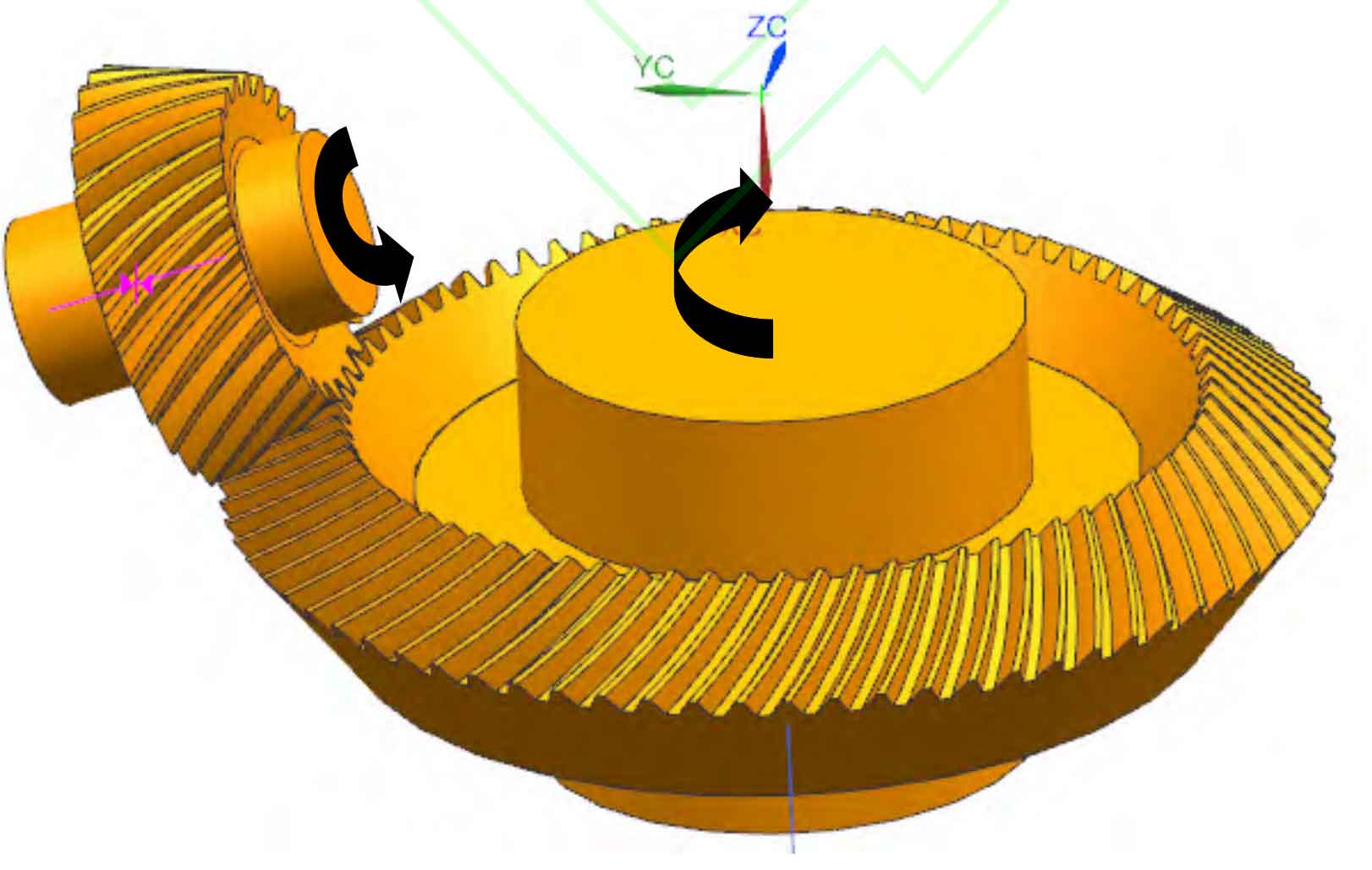
The UDF (User defined function) function is used in Fluent to set the grid, and the movement of the determined grid is displayed by specifying the wall rotation speed of the spiral bevel gear pair and shaft, as shown in the figure. Driven by the UDF function, the driving wheel and driven wheel rotate around the axis, where the speed of the small wheel is 20900r/min, the speed of the big wheel is 7626r/min, and the direction is as shown in figure, The mesh update process is automatically completed by Fluent according to the change of the boundary in each iteration step. In the dynamic mesh setting, turn on Remshing Smoothing, and all settings in spring smoothing remain default. In the mesh reconstruction, turn on the size function and set the minimum reconstruction size as the minimum mesh cell size of the gearbox. Consider that the mesh on the deformation edge interface turns on Local Face, The rest remain default.
Second order upwind discrete format is selected for momentum equation, and first order upwind discrete format is selected for turbulent kinetic energy and turbulent dissipation to improve calculation speed and accuracy. At the same time, the relaxation factor is adjusted appropriately to improve the convergence. The time step of transient analysis is set as 2e-6, and the steps are 6000. After initialization, iterative solution is performed.