1. Introduction

Bevel gears are widely used in mechanical transmissions with intersecting shafts due to their high efficiency, stability, convenience, and high torque-bearing capacity. However, they are prone to failure in closed and heavy-load conditions, which may lead to property loss and even casualties. Traditional fault diagnosis methods rely too much on prior knowledge and are time-consuming and labor-intensive. Convolutional neural networks (CNNs) have been proposed to solve the problems of traditional methods, but they require a large number of samples for training. When the samples are insufficient, the generalization ability of the model decreases. Therefore, the problem of insufficient types and data of fault samples is a problem that needs to be considered in the field of mechanical fault diagnosis. Transfer learning can overcome the difficulty of deep learning requiring a large amount of data by transferring knowledge learned in the source domain to the target domain. However, there are still two problems in transfer learning: overfitting and single feature of samples. To solve these problems, this paper proposes a bevel gear fault diagnosis method based on few samples, which uses sliding window overlapping sampling to expand the dataset, builds a 1D CNN model for bevel gear fault diagnosis, and realizes fault diagnosis under variable speed conditions through model transfer.

2. Convolutional Neural Network and Transfer Learning

2.1 Convolutional Neural Network

A convolutional neural network is a deep learning feedforward neural network that classifies input information invariantly according to the hierarchical structure. It mainly includes convolutional layers, pooling layers, fully connected layers, and output layers.

2.1.1 Convolutional Layers and Pooling Layers

The convolutional kernels in the convolutional layer traverse the input data to extract information features, which have the advantages of sparse connection and shared weights. The output of the convolutional layer is calculated as follows:

where α is the weight matrix, Xi is the output matrix of the i-th layer, f is the activation function, Xi-1 is the input matrix of the i-th layer, and b is the bias matrix.
After the input data is extracted by the convolutional layer, the pooling layer filters and selects features, extracting the maximum or mean value of multiple convolutional features within the region. The maximum pooling can obtain features independent of the position, and its calculation formula is as follows:

where Pki(j) is the j-th pooling output value of the k-th feature matrix of the i-th layer, qki(t) is the t-th value of the region processed by the i-th pooling kernel of the k-th feature matrix of the i-th layer, and s is the width of the pooling region.

2.1.2 Fully Connected Layers and Output Layers

The fully connected layer integrates the highly abstract features obtained after multiple convolutions and poolings of the input data and learns the nonlinear equation in the invariant low-dimensional space provided by the convolutional layer. The output layer classifies according to the probability obtained by the fully connected layer. The process operation is expressed as follows:

where  is the input value of the fully connected layer, that is, the feature matrix transmitted from the last convolutional layer, G is the output of the fully connected layer, b is the weight vector, and  is the bias vector. The output layer after the fully connected layer usually uses the Softmax function to convert the input of this layer into a probability distribution with a sum of 1 to prepare for the later target classification and recognition.

2.1.3 Activation Layers

The activation layer is often located behind the convolutional layer or the fully connected layer, and the activation function in the activation layer performs a nonlinear mapping on the output feature matrix of the convolutional layer to enhance the nonlinear ability of the convolution. In CNNs, three activation functions, ReLU, Tanh, and Sigmoid, are usually used to map the output features. Because the ReLU function has the characteristics of accelerating convergence and overcoming gradient dispersion, it is widely used.

2.2 Transfer Learning

Transfer learning can extract knowledge from a domain with rich data in a known scene and improve the learning ability of the target domain in an environment with few samples, different scenes, and changing tasks. It is a method based on the commonality of information, scenes, and models, which applies the knowledge learned in a known domain to other domains.

3. Bevel Gear Fault Diagnosis Transfer Convolutional Neural Network Model

This paper proposes a 1CNN bevel gear fault diagnosis model. The model is built based on the Pytorch deep learning framework using Python and mainly consists of five alternating convolutional and pooling layers. It extracts the features of vibration data through deep-to-shallow convolutions and connects the Softmax output through the fully connected layer to complete classification and recognition, forming the fault diagnosis result.

3.1 Network Basic Structure

The model has 13 layers of structural parameter training layers and adopts a small and deep network training structure. The network basic structure consists of five convolutional layers, five pooling layers, two fully connected layers, and one output layer. The network directly convolves and pools the one-dimensional time-domain signal. The front convolutional layer uses a large-size convolutional kernel for convolution, and the size of the convolutional kernel decreases with the depth of the network, effectively reducing the workload and improving the operating efficiency. In the model, choosing different sizes of convolutional kernels helps to extract rich information features from the vibration input data and improve the classification performance of the fault diagnosis model. Therefore, in the five alternating convolutional and pooling layers, to avoid the interference of high-frequency noise and the loss of local features during the training process, the first convolutional layer selects a medium-sized convolutional kernel with a size of 64×1, and the sizes of the subsequent four convolutional kernels are all 3×1. A maximum pooling layer with a kernel size of 2×1 is connected immediately after each convolutional layer.

3.2 Model Transfer

The 1CNN transfer convolutional neural network model is based on the deep CNN and introduces the Dropout technique to control the node weights in the neural network, optimize the network structure, prevent overfitting, and reduce the model recognition ability. First, the collected original data is filtered by convolution (Conv) operation to obtain partial features, and then the feature normalization (BN) is performed. The maximum pooling layer (Pool) samples the data and outputs the maximum value. Then, a Dropout layer is introduced after the maximum pooling layer to reduce the dependence of network nodes on any input. The fully connected layer (FC) maps the learned feature representation to the sample label space, and the output layer Softmax obtains the category output probability. Finally, the parameters of each layer are updated based on the cross-entropy backpropagation algorithm. The network search method is used to optimize the parameters such as the number of network layers, the number and size of convolutional kernels, and the size of nodes in the fully connected layer.

3.3 Basic Process

The specific steps of the model transfer fault diagnosis based on the deep convolutional neural network are as follows:

1. Source domain and target domain data sampling: Read the acceleration vibration data of the bevel gear and intercept a reasonable number of sample points as a unit sample to ensure that the model can fully learn the data features without consuming too many resources.
2. Dataset division: Divide the collected original vibration signals, and divide the samples into training and test sets according to a certain proportion.
3. Network structure construction: Set the size, stride, and number of kernels of the convolutional and pooling layers, and determine the size of the kernels of the fully connected and output layers.
4. Network parameter selection: Use the Adam gradient descent algorithm and select parameters such as the training epochs, the number of iterations, the initial learning rate, and the batch size for each round of training.
5. Build a pre-trained model: Train the convolutional neural network on the source domain samples, perform gradient descent using the loss function, perform backpropagation of the network for normalization, and update the network parameters until the model training converges to obtain a diagnostic classification model.
6. Model transfer: Freeze the parameters of the M1 – M5 modules, optimize the parameters of the M6 module, and perform model transfer.
7. Fault classification: Input the test samples of the target domain into the optimized 1CNN diagnostic model to obtain the classification result.

4. Experimental Verification and Analysis

4.1 Experimental Simulation

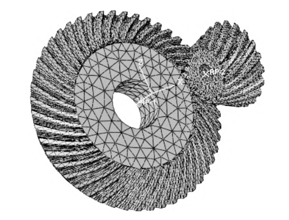
To verify the effectiveness of the model in bevel gear fault diagnosis, a comprehensive simulation experiment scheme was designed. The vibration data of the faulty bevel gear under different rotational speed conditions were collected to analyze the feasibility of improving the diagnostic accuracy under the condition of few sample data. The data source was the MFS mechanical fault comprehensive simulation test bench. The test bench mainly consisted of power, transmission, control, monitoring, and acquisition systems. The inverter controlled the operation of the variable speed motor, and the motor transmitted the torque and rotational speed to the drive shaft through the coupling. The pulley on the drive shaft transmitted the torque and rotational speed to the pulley on the bevel gear box, and the pulley drove the driving straight bevel gear with 18 teeth in the bevel gear box. The driven straight bevel gear with 27 teeth meshed with it and rotated. The driven bevel gear shaft overcame the resistance torque of the MTL10 – 5/8 magnetic brake. The resistance torque of the magnetic brake was adjusted by electromagnetic power, and the manual adjustable range was 0 – 5hp. IEPE piezoelectric acceleration sensors (model 1A116E) were installed at the center positions of the three surfaces of the bevel gear box. By replacing the driving bevel gears with different fault categories, the sensors collected the vibration signals of the bevel gear faults and transmitted the 3-channel fault data to the DH5922N dynamic signal test and analysis system.

4.2 Sample Generation

To study the influence of different numbers of training samples (with a fixed ratio of training to test samples) on the 1CNN transfer model, samples were constructed to explore the transfer learning ability. In the experiment, the straight bevel gear was taken as the research object, and the bevel gear faults such as broken teeth and missing teeth were simulated by electric discharge machining, as well as the normal state. The sampling frequency of the acceleration sensor was 20kHz. To simulate a specific load condition, the electromagnetic power was adjusted to 1hp. Since the rotational speed of the driving variable speed motor was controlled by the frequency converter, four frequency converter frequencies (10Hz, 20Hz, 30Hz, 40Hz) corresponding to four rotational speed conditions were selected in this experiment. Under a specific load, the three states of the bevel gear were simulated to run at four rotational speeds, and the vibration sensor collected the acceleration values for 1 minute, with a total of 12 groups of vibration data values. Each group of vibration data recorded 1,200,000 points. To ensure the learning effect and efficiency of the network, the number of sample data points was usually intercepted as the data of about two rotations of the bevel gear as one sample point. Therefore, 2048 data points were intercepted in turn as one sample, and a total of 480 samples were taken. The samples were randomly divided into 400 training samples and 80 test samples at a ratio of 5:1. The experimental sample data division.

4.3 Model Diagnosis

During the experiment, the vibration signals of the bevel gear in three states under four working conditions were collected. The time-domain waveforms of the A (10Hz) and B (20Hz) working conditions are shown in Figure 5. It can be seen that the waveform cannot confirm the operating condition and whether there is a fault, nor can it distinguish the fault state. To verify the fault recognition ability of the 1CNN network model under the condition of few samples, the time-domain signal was imported into the input layer for training to extract sample features under one rotational speed condition (source domain). After the model training was completed, it was transferred to another rotational speed condition (target domain), and the test samples under both working conditions were tested. The experiment was repeated 10 times, and the average value of the recognition accuracy of the test set under variable working conditions was taken as the experimental result.

4.4 Diagnostic Result Analysis

By changing the length of the sliding step, the training samples were expanded by the sliding window within 1 minute, and the influence of the difference in the number of samples between the unexpanded and expanded samples on the fault recognition accuracy of the test set under variable working conditions was compared. Due to space limitations, this paper only shows the source domain training model under the B rotational speed condition, which is transferred to the target domain under the A rotational speed condition and the samples in the test set are classified for fault recognition. The accuracy of the nine sample sets with the training and test sample ratios of 50:10, 100:20, 200:40, 300:60, 400:80, 485:197, 800:160, 1500:300, and 2500:500 generated by six sampling methods without sliding step and with 100, 200, 500, 1000, and 1600 sliding step length points is shown in Figure 6.
It can be found from the experimental data of the diagnostic experiment generated by different sliding steps that whether overlapping sampling is used or the sliding step length value is changed for sampling, the fault classification accuracy increases with the increase in the number of diagnostic samples. When the number of samples increases to a certain value, the accuracy improvement is not obvious. When no overlapping sampling is used, 682 samples are generated from the vibration data points recorded in 1 minute, and the accuracy is the highest at this time. When the sliding step length increases, the number of generated samples decreases. When the sliding step length reaches 1600, the accuracy basically does not change. For the other four sliding step lengths with overlapping sampling, the accuracy is improved to varying degrees. When the sliding step length is 100, the accuracy is improved by 12.85%. However, with the increase in the number of experimental samples, the model cannot converge in a short time, increasing the memory capacity and reducing the processing efficiency of the computer to a certain extent. Although reducing the sliding step length again can expand the samples, it will actually consume too much computing resources and slow down the model operation. Therefore, the overlapping sampling sliding window method can improve the accuracy of fault diagnosis classification with few samples.

4.5 Model Visualization

To intuitively show the application effect of the convolutional neural network in the fault recognition of the bevel gear under variable working conditions, taking the sliding window overlapping sampling with a sliding step length of 100 and 500 test samples as an example, the t-SNE dimensionality reduction was used to visualize the fully connected layer of the model, and the feature distributions of the test samples in the three states of the source and target domains were extracted, as shown in Figure 7.
The confusion matrix can be used to obtain the accuracy of fault classification in the test samples and analyze the specific prediction status of the test samples in the two domains. The confusion matrices of the source and target domains are shown in Figure 8. It can be seen from Figure 8 that the fault distributions of the test samples in the two domains basically coincide and are in an orderly state, and the fault category distinguishability is high. In the target domain test set, the three fault types are basically accurately classified. In particular, the missing tooth fault is completely recognized, and only 27 samples of the broken tooth fault are misidentified as normal. The overall fault classification accuracy can reach 97.73%.

5. Conclusion

In this paper, a 1D CNN transfer convolutional neural network model for bevel gear fault diagnosis was established to solve the problem of low fault recognition rate caused by a small number of samples in fault diagnosis of bevel gears under variable speed conditions. The overlapping sliding window sampling method was used to expand the samples, and the original input sample features were extracted. The bevel gear fault diagnosis experiment was carried out. The research shows that:

1. The convolutional neural network model with an appropriate interactive filter layer structure can realize the fault diagnosis classification of bevel gears under variable working conditions with few samples.
2. Under the condition of few samples, without changing the model parameters, using the overlapping sliding window sampling method to generate samples in both the source domain test set and the target domain test set can improve the accuracy of fault recognition.
3. When the sliding step length of the sliding window increases to a certain value, the number of expanded samples decreases, and the fault recognition rate cannot be further improved. A small sliding step length can continue the sample feature continuity and improve the diagnostic accuracy, but it will reduce the network operation efficiency to a certain extent. Only an appropriate sliding step length can achieve the optimal classification effect.
4. The transfer model learned from the samples generated by short-term faults can realize fault diagnosis under variable working conditions, which has great reference value in the practical application where faults cannot be reproduced.

In future research, we can further explore the optimization of the model structure and parameters, and study the combination of multiple fault diagnosis methods to improve the accuracy and reliability of bevel gear fault diagnosis. At the same time, we can also expand the application scenarios of the proposed method to other mechanical equipment and fault diagnosis fields to promote the development and application of fault diagnosis technology.