
Introduction
The machining accuracy of components forms the foundation for ensuring assembly quality in machine tools, particularly in bevel gear milling machines. This study focuses on establishing a geometric feature error model based on small displacement torsors (SDTs), analyzing error transmission properties in mating surfaces, and proposing a tolerance optimization framework. By integrating Monte Carlo simulation, response surface methodology, and reliability analysis, we aim to reduce manufacturing costs while maintaining assembly precision. Our work directly addresses challenges in bevel gear machining by optimizing tolerance design for spindle cutter disc components.
Geometric Feature Error Analysis
1.1 Error Modeling with SDTs
The SDT method describes rigid-body displacements using six parameters: three rotational (α, β, δ) and three translational (u, v, w). For conical surfaces, error boundaries are derived from tolerance zones. Consider a conical surface with radius R, height h, and taper 1:n. The upper (ZU) and lower (ZL) tolerance boundaries are:{2ny+z=2n(R+TU)2ny+z=2n(R−TL)
where TU and TL are upper and lower deviations. The SDT parameters for the conical surface are constrained by:⎩⎨⎧−h2+(2nh+T)2Th≤α≤h2+(2nh)2Th−TL≤v≤TU
Here, T=TU+TL. Similar models apply to cylindrical and planar features (Table 1).
Table 1: Error constraints for geometric features
| Feature | SDT Parameters | Constraints |
|---|---|---|
| Cylindrical | (α,β,0,u,v,0) | −2hTp+TF≤α≤2hTp+TF |
| Planar | (α,β,0,0,0,w) | −TL−To≤xβ+yα+w≤TU |
| Conical | (α,β,0,u,v,0) | R−TL−2nh≤α−2n(1+2nα)z+v≤R+TU |
1.2 Monte Carlo Simulation for Error Parameter Estimation
Monte Carlo simulation generates random error samples within tolerance bounds. Assuming normal distribution for errors, the mean (μ) and standard deviation (σ) are:μ^=2Ng1i=1∑2Ngki,σ^2=2Ng1i=1∑2Ng(ki−μ^)2
where k=α,β,u,v,w. The actual variation bandwidth is:Di=G6σ^i(G=1 for normal distribution)
1.3 Response Surface Methodology for Tolerance-Function Relationships
A quadratic polynomial models the relationship between tolerance T and error bandwidth Dj:Dj=c0+c1T1+c2T2+c3T12+c4T1T2+c5T22
Coefficients c0–c5 are determined via least squares. The coefficient of determination R2 validates model accuracy.
Assembly Error Transmission Modeling
2.1 Mating Surface Error Analysis
For conical mating surfaces, error transmission involves three components:
- Part Errors: Axis deviations due to manufacturing.
- Assembly Errors: Axial misalignment from clearance S.
- Constraint Propagation: Strong/weak constraints in serial/parallel mating.
The error transmission matrix for conical mating is:M34=10−β34001α340β34−α3410u34v3401
where α34 and u34 are derived from part and assembly errors.
Table 2: Error transmission properties of mating surfaces
| Mating Type | Strong Constraints | Weak Constraints | Unconstrained |
|---|---|---|---|
| Planar Non-Fixed | α,β,w | — | δ,u,v |
| Cylindrical Clearance | — | α,β,u,v | δ,w |
| Conical Clearance | — | α,β,u,v,w | δ |
2.2 Parallel Mating of Conical and Planar Surfaces
In bevel gear spindle assemblies, conical and planar surfaces often mate in parallel. The combined error transmission matrix is:Mparallel=Mconical⊗Mplanar
Key steps include:
- Hierarchical Constraints: Conical surfaces dominate positioning.
- Interference Check: Adjust tolerances if weak/strong constraints conflict.
Tolerance Optimization Framework
3.1 Reliability Analysis
The system reliability function g(T)=r−R(T) evaluates whether assembly precision R(T) meets threshold r. Monte Carlo simulations compute failure probability:Pf=NtotalNfail
where Nfail is the count of g(T)<0.
3.2 Cost-Driven Tolerance Optimization
The optimization model minimizes machining cost C(T) subject to reliability and tolerance hierarchy constraints:⎩⎨⎧minC(T)=∑i=1t(5.026e−15.8903Ti+0.3927Ti+0.1176Ti)s.t. R(T)≥97%Ts<Tp<TD(for hierarchical tolerances)
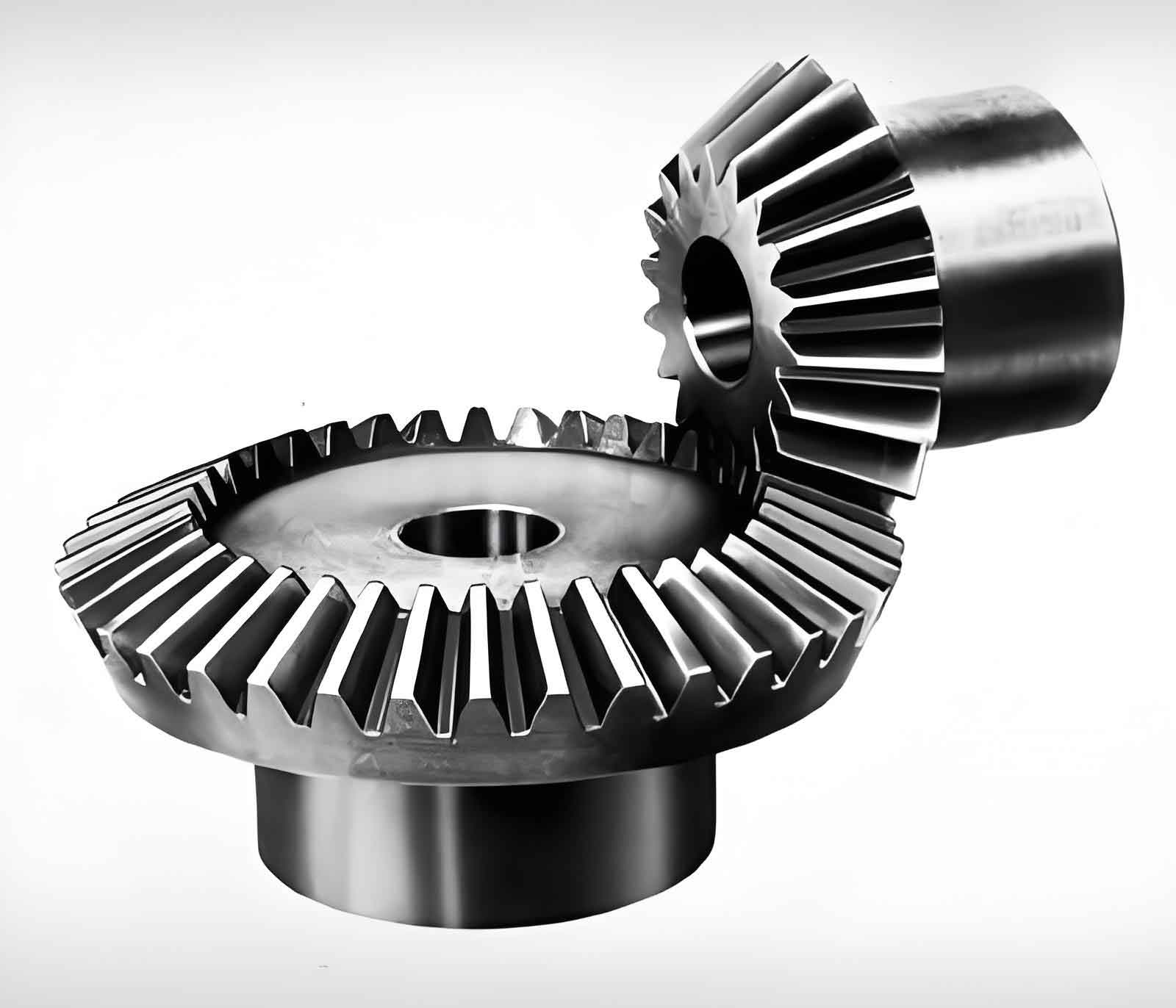
Case Study: Bevel Gear Spindle Cutter Disc
4.1 Error Transmission Model
The spindle-cutter assembly includes cylindrical, conical, and planar mating (Figure 5). Key tolerances include:
- Cylindrical Bore: Size (T1), cylindricity (T2), axis position (T3).
- Conical Shaft: Size (T7), taper (n), axis straightness (T4).
- Planar Face: Size (T9), perpendicularity (T10).
The cumulative error matrix is:Massembly=ED1⋅Mbc⋅ED2⋅Mde⋅ED3⋅Mfg
where ED1,ED2,ED3 represent error matrices for cylindrical, conical, and planar components.
4.2 Optimization Results
After applying the framework:
- Cost Reduction: 8.36% lower machining costs.
- Reliability: 97.3% assembly precision reliability.
- Critical Tolerances: Conical size (T7) and planar perpendicularity (T10) dominated cost-reliability trade-offs.
Conclusion
This study presents a systematic approach to modeling and optimizing assembly errors in bevel gear milling machines. By integrating SDT-based error analysis, Monte Carlo simulation, and cost-driven optimization, we achieved significant cost savings without compromising precision. Future work will extend this framework to dynamic error analysis during machining.