
1. Introduction
Straight bevel gears are critical components in power transmission systems, particularly in applications requiring orthogonal shaft arrangements. Their dynamic behavior under operational conditions—such as amplitude jumps, multi-solution coexistence, and tooth surface impacts—has significant implications for system reliability and longevity. This study investigates the nonlinear dynamic characteristics of a straight bevel gear system with backlash, focusing on parameter sensitivity and solution domain boundary structures in two-parameter planes. By combining harmonic balance methods, Broyden quasi-Newton algorithms, and pseudo-arclength continuation techniques, we analyze how key parameters—backlash, time-varying stiffness, static transmission error, and load—affect system dynamics.
2. Dynamic Model of Straight Bevel Gear Systems
2.1 Governing Equations
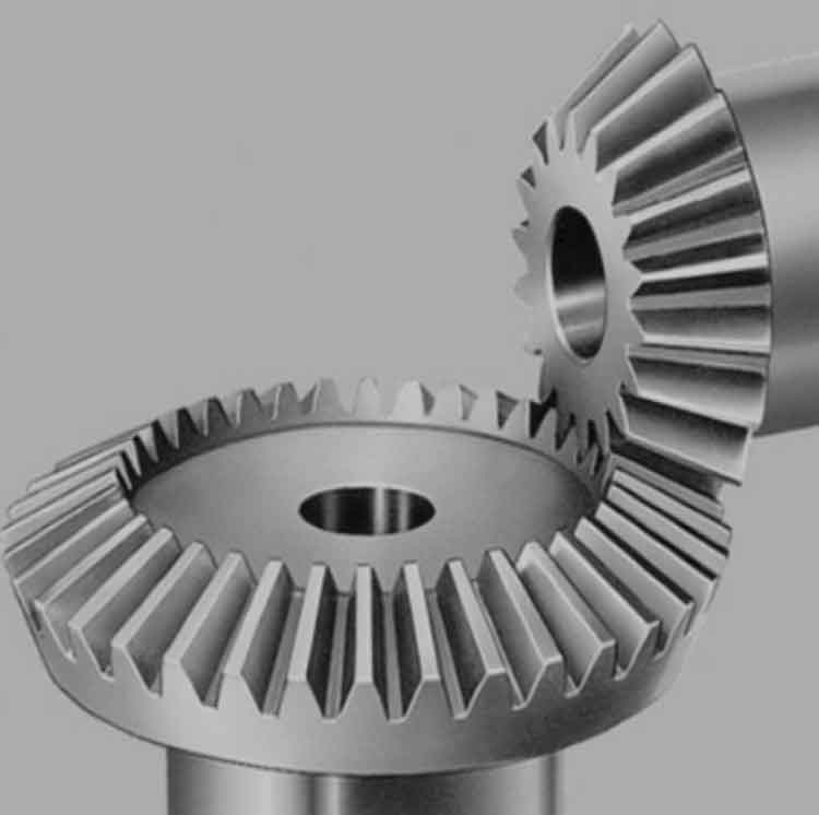
The 7-degree-of-freedom (DOF) dynamic model of a straight bevel gear system (Figure 1) accounts for translational and rotational motions of the gears. The relative displacement along the meshing line, ΛnΛn, is defined as:Λn=(X1−X2)a1−(Y1−Y2)a2−(Z1−Z2+r1θ1−r2θ2)a3−en(t),Λn=(X1−X2)a1−(Y1−Y2)a2−(Z1−Z2+r1θ1−r2θ2)a3−en(t),
where a1=cosδ1sinαna1=cosδ1sinαn, a2=cosδ1cosαna2=cosδ1cosαn, a3=cosαna3=cosαn, and en(t)en(t) represents static transmission error.
The meshing force FnFn and its components are:Fn=kn(t)f(Λn)+cnΛ˙n,Fn=kn(t)f(Λn)+cnΛ˙n,{Fx=a2Fn,Fy=a3Fn,Fz=a3Fn,⎩⎨⎧Fx=a2Fn,Fy=a3Fn,Fz=a3Fn,
where kn(t)kn(t) is time-varying stiffness, and f(Λn)f(Λn) is the backlash function:f(Λn)={Λn−bnΛn>bn,0∣Λn∣≤bn,Λn+bnΛn<−bn.f(Λn)=⎩⎨⎧Λn−bn0Λn+bnΛn>bn,∣Λn∣≤bn,Λn<−bn.
2.2 Dimensionless Equations
Normalizing variables (xj=Xj/bhxj=Xj/bh, λ=Λn/bhλ=Λn/bh) yields dimensionless equations:{x¨1+2ξx1x˙1+kx1x1=Fx,y¨1+2ξy1y˙1+ky1y1=Fy,z¨1+2ξz1z˙1+kz1z1=Fz,θ¨1=T1−Fxr1/J1,x¨2+2ξx2x˙2+kx2x2=−Fx,y¨2+2ξy2y˙2+ky2y2=−Fy,z¨2+2ξz2z˙2+kz2z2=−Fz,θ¨2=T2+Fxr2/J2.⎩⎨⎧x¨1+2ξx1x˙1+kx1x1=Fx,y¨1+2ξy1y˙1+ky1y1=Fy,z¨1+2ξz1z˙1+kz1z1=Fz,θ¨1=T1−Fxr1/J1,x¨2+2ξx2x˙2+kx2x2=−Fx,y¨2+2ξy2y˙2+ky2y2=−Fy,z¨2+2ξz2z˙2+kz2z2=−Fz,θ¨2=T2+Fxr2/J2.
3. Methodology: Harmonic Balance and Continuation
3.1 Harmonic Balance Formulation
Assuming steady-state responses dominated by the fundamental harmonic, displacements are approximated as:xi=xmi+xcicos(Ωτ)+xsisin(Ωτ),xi=xmi+xcicos(Ωτ)+xsisin(Ωτ),
where xmixmi, xcixci, and xsixsi represent mean, cosine, and sine components. The backlash function f(λ)f(λ) is expanded using Fourier series:f(λ)=Nmixmi+Naixcicos(Ωτ)+Naixsisin(Ωτ),f(λ)=Nmixmi+Naixcicos(Ωτ)+Naixsisin(Ωτ),
with describing functions NmiNmi and NaiNai:{Nmi=1+xai[G(μi+)−G(μi−)]2xmi,Nai=1−[H(μi+)−H(μi−)]2,{Nmi=2xmi1+xai[G(μi+)−G(μi−)],Nai=21−[H(μi+)−H(μi−)],
where μi±=(±b−xmi)/xaiμi±=(±b−xmi)/xai, and G(μ)G(μ), H(μ)H(μ) are piecewise functions.
3.2 Broyden Quasi-Newton and Pseudo-Arclength Continuation
Nonlinear algebraic equations derived from harmonic balance are solved using:
- Broyden’s Method: Updates Jacobian approximations iteratively.
- Pseudo-Arclength Continuation: Traces solution branches globally, capturing multi-value responses and bifurcations.
4. Results: Parameter Sensitivity and Solution Domains
4.1 Amplitude Jump and Multi-Solution Phenomena
Figure 2 illustrates amplitude jumps in the meshing frequency (Ω∈[0.3,1.5]Ω∈[0.3,1.5]) and shaft frequency resonance regions. Key observations include:
- Stiffness Softening: Red curves shift toward lower frequencies.
- Backlash Threshold: For b>0.98b>0.98, jumps stabilize (Figure 3a).
- Time-Varying Stiffness: Amplitude jumps intensify with higher aa (Figure 3b).
4.2 Tooth Surface Impact Criteria
Impact states II are classified as:I={0λa−λs>b,1(λa−λs<b)∩(λa+λs>b),2(λa−λs<b)∩(λa+λs<b).I=⎩⎨⎧012λa−λs>b,(λa−λs<b)∩(λa+λs>b),(λa−λs<b)∩(λa+λs<b).
Coexistence of multi-solutions (n=1,2n=1,2) and impacts (I=0,1,2I=0,1,2) is denoted as n/In/I.
4.3 Parameter Solution Domains
Tables 1–4 summarize n/In/I state distributions in (Ω,b)(Ω,b), (Ω,a)(Ω,a), (Ω,fe)(Ω,fe), and (Ω,fm)(Ω,fm) planes.
Table 1: n/In/I States in (Ω,b)(Ω,b) Plane
| Backlash (bb) | Frequency (ΩΩ) | Dominant n/In/I States |
|---|---|---|
| b<0.2b<0.2 | Ω≈1.2Ω≈1.2 | 2/1-2, 2/0-1 |
| 0.2<b<0.980.2<b<0.98 | Ω≈0.6Ω≈0.6 | 1/1, 2/0-2 |
| b>0.98b>0.98 | All ΩΩ | 1/0, 1/1 |
Table 2: n/In/I States in (Ω,a)(Ω,a) Plane
| Stiffness (aa) | Frequency (ΩΩ) | Dominant n/In/I States |
|---|---|---|
| a<0.25a<0.25 | Ω≈1.2Ω≈1.2 | 2/1-2 |
| 0.25<a<0.40.25<a<0.4 | Ω≈0.6Ω≈0.6 | 1/1 |
| a>0.4a>0.4 | All ΩΩ | 1/0 |
5. Discussion and Engineering Implications
- Backlash Control: Small backlash (b<0.2b<0.2) exacerbates tooth impacts, while b>0.98b>0.98 stabilizes dynamics.
- Stiffness Design: Time-varying stiffness significantly affects meshing frequency jumps but has minimal impact on shaft frequency responses.
- Error and Load: High static errors (fefe) and light loads (fmfm) amplify nonlinearities, necessitating precision manufacturing and robust loading.
6. Conclusion
This study establishes a comprehensive framework for analyzing straight bevel gear dynamics using harmonic balance and continuation methods. Key findings include:
- Parameter Thresholds: Critical values (e.g., b=0.98b=0.98, a=0.4a=0.4) demarcate stable and unstable regimes.
- Solution Domains: Multi-solution and impact states are mapped in parameter planes, guiding gear design optimization.
- Practical Guidelines: Increasing backlash beyond 0.98 or stiffness beyond 0.4 suppresses nonlinear jumps and tooth impacts.