
Ensuring the operational reliability of shearers is paramount for efficient and safe coal production. Among critical components, the gears within the shearer’s cutting section are highly susceptible to failure due to harsh operating conditions and heavy loads. Traditional fault diagnosis methods often struggle with complex feature extraction and accurate prediction. Deep learning offers a promising solution by autonomously learning intricate patterns from raw sensor data, enabling more effective gear failure prediction and classification. This study focuses on developing a deep learning-based model for predicting gear failure in the cutting section of an MG1000/2500-WD shearer.
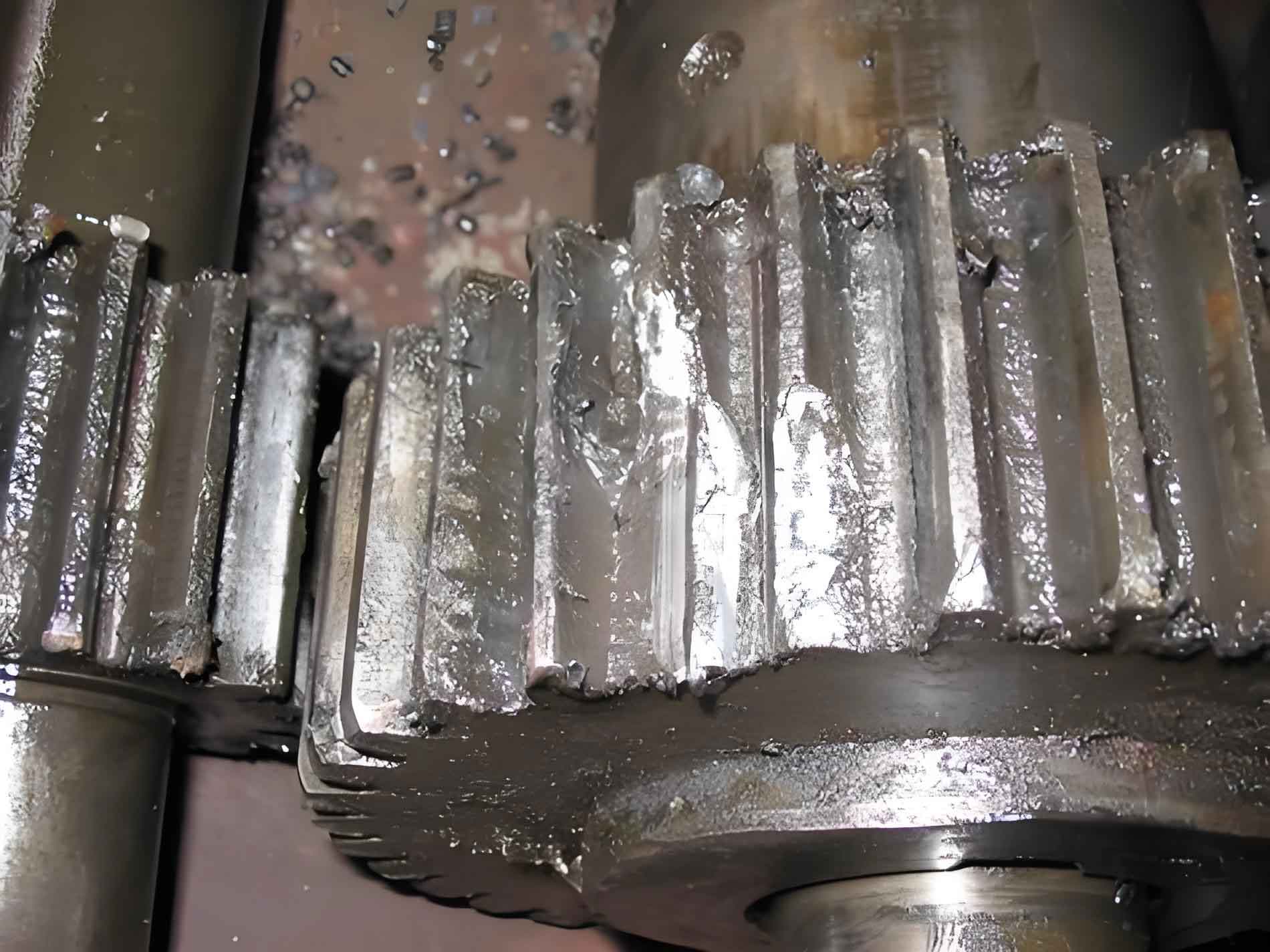
The shearer’s cutting section, primarily responsible for coal cutting and loading, houses complex gear transmission systems crucial for power transmission. These gears operate under extreme stresses, leading to various failure modes. Common gear failure types include:
- Gear tooth breakage: Often caused by fatigue under cyclic loading or impact overload during operations like cutting hard rock inclusions.
- Pitting and spalling: Surface fatigue failures resulting from repeated Hertzian contact stresses, exacerbated by inadequate lubrication or contamination.
- Scoring/scuffing: Caused by lubrication breakdown leading to high friction, localized welding, and tearing of tooth surfaces.
- Abrasive wear: Accelerated surface material removal due to hard contaminants like coal dust or grit in the lubricant.
- Plastic deformation (ridging, indentation): Occurs under severe overload conditions exceeding the material’s yield strength.
Accurately predicting these gear failure modes is critical for proactive maintenance, preventing catastrophic breakdowns, and minimizing downtime. The complex nature of vibration signals generated by gear meshing and incipient faults necessitates sophisticated analysis techniques.
Convolutional Neural Networks (CNNs) excel at learning hierarchical features from structured data like time-series signals. A Deep Convolutional Neural Network (D-CNN) architecture is employed here for gear failure prediction. Its core components are:
- Input Layer: Accepts preprocessed 1D vibration signal segments. Sliding window sampling with overlap generates sufficient training samples:
$$ n = \left\lfloor \frac{L – 1}{l \times \delta} \right\rfloor $$
where \(L\) is the total signal length, \(l\) is the sample length, \(\delta\) is the overlap ratio, and \(\lfloor \cdot \rfloor\) denotes the floor function. - 1D Convolutional Layers: Multiple layers perform feature extraction using learnable kernels/filters. The operation for the \(l^{th}\) layer’s \(j^{th}\) feature map is:
$$ x_j^l = f\left( \sum_{i \in M_j} x_i^{l-1} \ast k_{ij}^l + b_j^l \right) $$
where \(x_j^l\) is the output, \(x_i^{l-1}\) is the input from the previous layer, \(k_{ij}^l\) is the convolution kernel, \(\ast\) denotes convolution, \(b_j^l\) is the bias, \(M_j\) is the input feature map set, and \(f(\cdot)\) is the activation function. The Rectified Linear Unit (ReLU) activation is used for its efficiency and sparsity induction:
$$ \text{ReLU}(x) = \max(0, x) $$ - 1D Pooling Layers (Max Pooling): Reduce feature map dimensionality and provide translational invariance. For the \((l+1)^{th}\) layer’s \(j^{th}\) feature map:
$$ P_j^{l+1}(i) = \max_{(i-1)W +1 \leq t \leq iW} \{ a_j^l(t) \} $$
where \(W\) is the pooling window width, and \(a_j^l(t)\) is the activation at position \(t\). - Dropout Layer: Mitigates overfitting by randomly dropping neurons (rate=0.5) during training. The output \(O_i\) for neuron \(i\) is:
$$ O_i = X_i \cdot a\left( \sum_{k=1}^{d} w_k x_k + b \right) $$
where \(X_i\) is a Bernoulli random variable (\(P(X_i=1) = q = 0.5\)), \(a(\cdot)\) is the activation function, \(d\) is the input dimension, \(w_k\) are weights, and \(b\) is the bias. - Fully Connected (FC) Layers: Integrate high-level features extracted by preceding layers. The output \(z_j^{l+1}\) of the \((l+1)^{th}\) layer’s \(j^{th}\) neuron is:
$$ z_j^{l+1} = \sum_{i=1}^{n} w_{ij}^l P_j^l + b_j^l $$
where \(w_{ij}^l\) are weights connecting the \(i^{th}\) neuron in layer \(l\) to the \(j^{th}\) neuron in layer \(l+1\), and \(P_j^l\) is the input from the previous layer. - Output Layer (Softmax): Provides probability distribution over the predicted gear health states (e.g., Normal, Wear, Pitting, Broken Tooth, Crack). The probability \(q(z_j)\) for class \(j\) is:
$$ q(z_j) = \text{Softmax}(z_j) = \frac{\exp(z_j)}{\sum_{n=1}^{N} \exp(z_n)} $$
where \(z_j\) is the input to the Softmax function for class \(j\), and \(N\) is the total number of classes.
The model is trained using the Adam optimizer to minimize the Categorical Cross-Entropy loss function \(L\):
$$ L = -\frac{1}{m} \sum_{k=1}^{m} \sum_{j} p_j^k \log(q_j^k) $$
where \(m\) is the mini-batch size, \(p_j^k\) is the true probability (1 for the true class, 0 otherwise), and \(q_j^k\) is the predicted probability for class \(j\) in sample \(k\).
The D-CNN algorithm workflow involves data acquisition, preprocessing (normalization, segmentation), model training (80% data), hyperparameter tuning using a validation set (10% data), and final evaluation on a separate test set (10% data). Batch processing (size=64) and early stopping prevent overfitting and ensure efficient training.
Experimental validation utilized vibration data from a gear test rig simulating shearer operating conditions. Data included various gear health states under different loads and damage severities. Key datasets are summarized below:
| State ID | Gear Health State | Load (hp) | Damage Size (mm) | Sample Length | # Samples |
|---|---|---|---|---|---|
| 0 | Normal | 0 | 0 | 1000 | 100 |
| 1 | Inner Race Fault | 1 | 7 | 1000 | 100 |
| 2 | Outer Race Fault | 1 | 7 | 1000 | 100 |
| 3 | Rolling Element Fault | 1 | 7 | 1000 | 100 |
| 4 | Inner Race Fault | 2 | 14 | 1000 | 100 |
| 5 | Outer Race Fault | 2 | 14 | 1000 | 100 |
| 6 | Rolling Element Fault | 2 | 14 | 1000 | 100 |
| 7 | Inner Race Fault | 3 | 21 | 1000 | 100 |
| 8 | Outer Race Fault | 3 | 21 | 1000 | 100 |
| 9 | Rolling Element Fault | 3 | 21 | 1000 | 100 |
Sliding window segmentation (overlap ratio δ=0.05) expanded the original 1000 samples into 2455 samples for model training and testing. The D-CNN model architecture and training parameters were configured as follows:
| Layer Type | Specification | Hyperparameter | Value |
|---|---|---|---|
| Input | 1D Signal Segment | Input Shape | (1000, 1) |
| Conv1D | Kernels: 64, Size: 64 | Activation | ReLU |
| MaxPooling1D | Pool Size: 3 | Stride | 3 |
| Conv1D | Kernels: 32, Size: 32 | Activation | ReLU |
| MaxPooling1D | Pool Size: 3 | Stride | 3 |
| Conv1D | Kernels: 16, Size: 16 | Activation | ReLU |
| MaxPooling1D | Pool Size: 3 | Stride | 3 |
| Flatten | – | – | – |
| Dropout | – | Rate | 0.5 |
| Dense (FC) | 100 Neurons | Activation | ReLU |
| Dense (Output) | 10 Neurons | Activation | Softmax |
| – | Optimizer | Adam | – |
| – | Loss Function | Categorical Cross-Entropy | – |
| – | Learning Rate | 0.001 | – |
| – | Batch Size | 64 | – |
| – | Epochs | 100 | – |
Training demonstrated rapid convergence, with training and validation accuracy exceeding 99% and loss approaching zero within 100 epochs, indicating effective learning without significant overfitting. The model achieved an overall gear failure identification rate of 98.71% on the test set. Performance metrics for classifying specific shearer cutting section gear states are detailed below:
| State ID | Gear Health State | Precision (%) | Recall (%) |
|---|---|---|---|
| 0 | Normal | 96.32 | 98.27 |
| 1 | Wear | 99.21 | 100.00 |
| 2 | Pitting | 98.34 | 96.67 |
| 3 | Broken Tooth | 100.00 | 99.45 |
| 4 | Crack | 100.00 | 100.00 |
| Average | – | 98.78 | 98.88 |
High precision and recall values (averaging 98.78% and 98.88%, respectively) confirm the model’s strong capability to accurately identify both normal and faulty gear conditions, minimizing false positives and false negatives. Visualization of the learned features in the final fully connected layer using t-SNE showed clear clustering of different gear health states, demonstrating the model’s discriminative power.
To benchmark performance, the D-CNN model was compared against established deep learning models: Deep Neural Network (DNN), Stacked Autoencoder (SAE), and Deep Belief Network (DBN). All models were trained and tested on the identical dataset. The D-CNN model significantly outperformed the alternatives in gear failure identification accuracy, particularly for challenging fault types like inner and outer race faults under varying damage sizes and loads. The D-CNN also achieved the highest precision in distinguishing normal gear operation from various failure states.
| Model | Description | Overall Test Accuracy (%) | Precision (Normal vs. Fault) (%) |
|---|---|---|---|
| DNN | Input(1024) – FC(100) – FC(50) – Output(10) | 84.38 | 84.38 |
| SAE | Input(1024) – FC(512) – FC(256) – FC(128) – Output(10) | 87.33 | 87.33 |
| DBN | Input(1024) – FC(100) – FC(50) – Output(10) | 85.47 | 85.47 |
| D-CNN (Proposed) | Architecture as per Table 2 | 98.71 | 98.13 |
The proposed D-CNN model demonstrates exceptional efficacy in predicting gear failure within the shearer cutting section, achieving a high identification rate of 98.71%. Its superior performance, evidenced by high precision (98.78%) and recall (98.88%), surpasses traditional deep learning models like DNN, SAE, and DBN. This accuracy stems from the model’s ability to autonomously learn discriminative spatio-temporal features directly from raw vibration signals through deep convolutional layers, effectively capturing the complex patterns associated with incipient and developed gear failure. The integration of dropout regularization successfully mitigated overfitting, ensuring robust generalization. Future work will focus on incorporating multi-sensor data fusion (e.g., vibration, temperature, acoustic emission) and exploring transfer learning to adapt the model to varying shearer models and operational conditions, further enhancing the robustness and applicability of gear failure prediction for proactive maintenance in coal mining operations.