
In this study, we delve into the dynamic characteristics of electromechanical integrated electromagnetic worm gear drive systems, focusing on their parameter vibration responses due to time-varying electromagnetic meshing stiffness. The worm gear drive system represents a novel coupling mechanism that integrates traditional worm drive technology with electromagnetic actuation, offering advantages such as compact structure, controllable output torque and speed, and reduced wear and noise. However, the periodic variation in the number of meshing magnetic poles introduces time-dependent stiffness, leading to parameter vibrations that can significantly impact system performance, including resonance phenomena. Our aim is to develop a comprehensive model, derive analytical solutions using perturbation methods, and analyze free vibration, primary resonance, and combination resonance behaviors. We will employ multiple scales method to obtain approximate solutions and present results in both time and frequency domains, emphasizing the role of system natural frequencies and their combinations with meshing frequencies. Throughout this article, we will frequently refer to the worm gear drive system to underscore its centrality in our analysis.
The structure of an electromechanical integrated worm gear drive system typically consists of an electromagnetic worm with three-phase alternating current coils and a worm wheel equipped with permanent magnet teeth, all mounted within a housing. When energized, the coils generate a rotating magnetic field that drives the worm wheel, enabling torque transmission without physical contact. This non-contact operation reduces mechanical fatigue and lubrication issues, but the varying meshing stiffness—a consequence of alternating between one and two pairs of magnetic teeth in engagement—introduces parametric excitations. To illustrate, consider the following schematic representation of a typical worm gear drive setup:
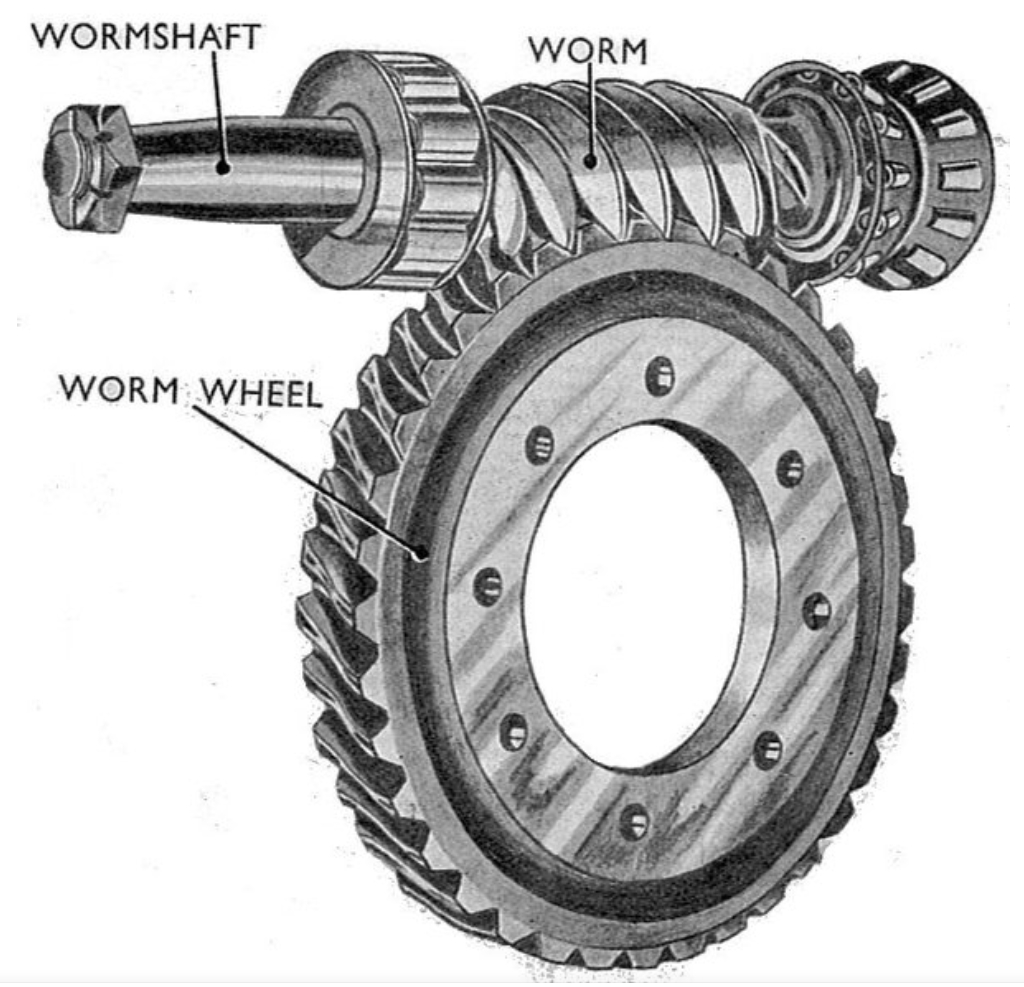
This image depicts the essential components of a worm gear drive, highlighting the interaction between the worm and wheel. In our system, the electromagnetic nature adds complexity, as the meshing stiffness depends on factors like current intensity, inductance, and geometric parameters. We begin by deriving the expression for time-varying electromagnetic meshing stiffness, which serves as the foundation for our dynamic model.
The electromagnetic meshing stiffness, \( k(t) \), varies periodically with the relative rotation angle \(\theta\) between the worm coils and worm wheel teeth. For a system with 8 permanent magnet teeth on the worm wheel and a wrap angle of 80°, the meshing alternates between 1 and 2 pairs of teeth. The stiffness function over one meshing period \( T_p \) can be expressed as:
$$ k(t) = \begin{cases}
k_{p1} & \text{for } \left(m – \frac{2 – \varepsilon_p}{2}\right)T_p \leq t < \left(m + \frac{2 – \varepsilon_p}{2}\right)T_p \\
k_{p2} = 2k_{p1} & \text{for } \left(m + \frac{2 – \varepsilon_p}{2}\right)T_p \leq t < \left(m + \frac{\varepsilon_p}{2}\right)T_p
\end{cases} $$
where \( m \) is an integer representing the meshing cycle number, \( \varepsilon_p \) is the contact ratio, and \( k_{p1} \) is the stiffness for single-tooth engagement. The stiffness \( k_{p1} \) is given by:
$$ k_{p1} = K \frac{I_s^2 z^2 L_1}{2r^2} \cos\left(z \theta + \frac{\phi_v}{3n_1 p}\right) \bigg|_{\theta = \theta_0} $$
with \( K = \cos\left(\frac{\phi_v}{3n_1 p}\right) + 4\cos\left(\frac{\phi_v}{6n_1 p}\right) + 3 \), where \( I_s \) is the current intensity, \( z \) is the number of teeth, \( L_1 \) is the average inductance, \( r \) is the worm wheel radius, \( \phi_v \) is the wrap angle, \( \theta_0 \) is the static rotation angle, \( n_1 \) is the number of phases, and \( p \) is the pole number. The contact ratio \( \varepsilon_p \) and meshing period \( T_p \) are defined as:
$$ T_p = \frac{2\pi}{z \omega_p}, \quad \varepsilon_p = \frac{16}{9} $$
where \( \omega_p \) is the worm wheel angular velocity. The time-varying stiffness function is even and can be expanded into a Fourier series in complex form:
$$ k(t) = \sum_{n=-\infty}^{+\infty} k_n e^{i \left( \frac{2n\pi}{T_p} t \right)} $$
The Fourier coefficients are calculated as:
$$ k_0 = \frac{1}{T_p} \left( \int_{-(2-\varepsilon_p)T_p/2}^{(2-\varepsilon_p)T_p/2} k_{p1} \, dt + \int_{(2-\varepsilon_p)T_p/2}^{\varepsilon_p T_p/2} k_{p2} \, dt \right) = \varepsilon_p k_{p1} $$
$$ k_n = \frac{1}{T_p} \left( \int_{-(2-\varepsilon_p)T_p/2}^{(2-\varepsilon_p)T_p/2} k_{p1} e^{-i \left( \frac{2n\pi}{T_p} t \right)} \, dt + \int_{(2-\varepsilon_p)T_p/2}^{\varepsilon_p T_p/2} k_{p2} e^{-i \left( \frac{2n\pi}{T_p} t \right)} \, dt \right) = -\frac{k_{p1}}{n\pi} \sin\left( \frac{2n\pi}{9} \right) $$
Thus, the stiffness can be written as the sum of average stiffness \( \bar{k} \) and time-varying component \( \Delta k(t) \):
$$ k(t) = \bar{k} + \Delta k(t) = k_0 – \frac{k_{p1}}{\pi} \sum_{n=1}^{\infty} \frac{1}{n} \sin\left( \frac{2n\pi}{9} \right) \left( e^{i (n \omega_p t)} + e^{-i (n \omega_p t)} \right) $$
where \( \bar{k} = \frac{16}{9} k_{p1} \). This expression highlights the periodic nature of the stiffness in the worm gear drive system, which drives the parameter vibrations.
To model the dynamics, we use a lumped-parameter approach for the worm gear drive system. The equation of motion for the worm wheel’s torsional displacement \( x \) (linearized along the rotation axis) is:
$$ m \ddot{x} + c \dot{x} + k(t) x = \frac{\Delta T \cos(\omega t)}{r} $$
where \( m \) is the equivalent mass, \( c \) is the damping coefficient, \( \Delta T \) is the amplitude of output torque fluctuation, and \( \omega \) is the fluctuation frequency. Substituting the stiffness expression, we obtain:
$$ \ddot{x} + 2\zeta_0 \omega_0 \dot{x} + \omega_0^2 \left[ 1 – \varepsilon \sum_{n=1}^{\infty} b_n \left( e^{i (n \omega_p t)} + e^{-i (n \omega_p t)} \right) \right] x = \frac{T}{mr} $$
with \( \omega_0 = \sqrt{\bar{k}/m} \) as the natural frequency, \( \zeta_0 = c/(2\omega_0 m) \), \( \varepsilon = a_1 \), \( a_n = \frac{k_{p1} \sin(2n\pi/9)}{n\pi \omega_0^2} \), and \( b_n = a_n / a_1 \). The term \( T \) represents the torque input, and for simplicity, we often set \( T = \Delta T \cos(\omega t) \) for forced vibrations. This equation is a linear time-varying differential equation characteristic of parameter vibrations in worm gear drive systems.
We now proceed to analyze the free vibration response of the worm gear drive system. Setting the right-hand side to zero, the free vibration equation is:
$$ \ddot{x} + 2\varepsilon \zeta \omega_0 \dot{x} + \omega_0^2 \left[ 1 – \varepsilon \sum_{n=1}^{\infty} b_n \left( e^{i (n \omega_p t)} + e^{-i (n \omega_p t)} \right) \right] x = 0 $$
where we have scaled damping as \( \zeta = \varepsilon \zeta_0 \) to balance effects in perturbation analysis. We employ the method of multiple scales, introducing time scales \( T_0 = t \), \( T_1 = \varepsilon t \), and expressing the solution as an expansion in \( \varepsilon \):
$$ x = x_0(T_0, T_1) + \varepsilon x_1(T_0, T_1) + \varepsilon^2 x_2(T_0, T_1) + \cdots $$
Substituting into the equation and collecting terms of equal power in \( \varepsilon \), we derive a hierarchy of equations. The zeroth-order equation is:
$$ D_0^2 x_0 + \omega_0^2 x_0 = 0 $$
where \( D_k = \partial / \partial T_k \). Its solution is:
$$ x_0 = A(T_1) e^{i \omega_0 T_0} + \text{c.c.} $$
with c.c. denoting complex conjugate. The first-order equation is:
$$ D_0^2 x_1 + \omega_0^2 x_1 = -2D_0 D_1 x_0 – 2\zeta \omega_0 D_0 x_0 + \omega_0^2 x_0 \sum_{n=1}^{\infty} b_n \left( e^{i (n \omega_p t)} + e^{-i (n \omega_p t)} \right) $$
Eliminating secular terms yields the solvability condition:
$$ -2i \omega_0 A’ – 2i \zeta \omega_0^2 A = 0 $$
where \( A’ = dA/dT_1 \). Solving this gives:
$$ A = E_0 e^{-\zeta \omega_0 T_1} $$
with \( E_0 \) as a constant determined from initial conditions. For the worm gear drive system, \( E_0 \) can be related to the static torque \( T \) as \( E_0 = T / (\bar{k} r) \). Then, solving for \( x_1 \), we obtain the first-order approximation:
$$ x_1 = -\frac{\omega_0^2 E_0}{2} e^{-\zeta \omega_0 T_1} \sum_{n=1}^{\infty} b_n \left[ \frac{e^{i (n \omega_p + \omega_0) T_0}}{n \omega_p (n \omega_p + 2 \omega_0)} + \frac{e^{i (\omega_0 – n \omega_p) T_0}}{n \omega_p (n \omega_p – 2 \omega_0)} \right] + \text{c.c.} $$
Thus, the free vibration response up to first order is:
$$ x = E_0 e^{-\zeta \omega_0 T_1} e^{i \omega_0 T_0} – \varepsilon \frac{\omega_0^2 E_0}{2} e^{-\zeta \omega_0 T_1} \sum_{n=1}^{\infty} b_n \left[ \frac{e^{i (n \omega_p + \omega_0) T_0}}{n \omega_p (n \omega_p + 2 \omega_0)} + \frac{e^{i (\omega_0 – n \omega_p) T_0}}{n \omega_p (n \omega_p – 2 \omega_0)} \right] + \text{c.c.} + \cdots $$
This solution reveals that the free vibration of the worm gear drive system includes not only the natural frequency \( \omega_0 \) but also combination frequencies \( |\omega_0 \pm n \omega_p| \), unlike constant-coefficient linear systems. The damping causes amplitude decay over time. To quantify this, we consider a numerical example with parameters typical for a worm gear drive system, as shown in Table 1.
| Parameter | Symbol | Value |
|---|---|---|
| Number of teeth | \( z \) | 8 |
| Mass | \( m \) | 10 kg |
| Damping coefficient | \( c \) | 0.1 N·s/m |
| Rated torque | \( T \) | 200 N·m |
| Radius | \( r \) | 0.15 m |
| Static angle | \( \theta_0 \) | 0.0424° |
| Wrap angle | \( \phi_v \) | 80° |
| Current intensity | \( I_s \) | 100 A |
| Inductance | \( L_1 \) | 1.0 × 10⁻³ H |
| Meshing frequency | \( \omega_p \) | 160 rad/s |
| Torque fluctuation amplitude | \( \Delta T \) | 5 N·m |
Using these values, we compute the response. For instance, taking the first three terms in the series (n=1,2,3), the time-domain response shows harmonic decay, while the frequency-domain spectrum confirms peaks at \( \omega_0 \) and \( \omega_0 \pm n \omega_p \). This underscores the complexity of parameter vibrations in worm gear drive systems, where multiple frequency components coexist even in free vibration.
Next, we investigate the primary resonance of the worm gear drive system, occurring when the external torque fluctuation frequency \( \omega \) is close to the natural frequency \( \omega_0 \). The forced vibration equation is:
$$ \ddot{x} + 2\varepsilon \zeta \omega_0 \dot{x} + \omega_0^2 \left[ 1 – \varepsilon \sum_{n=1}^{\infty} b_n \left( e^{i (n \omega_p t)} + e^{-i (n \omega_p t)} \right) \right] x = \frac{\Delta T}{2mr} \left( e^{i \omega t} + e^{-i \omega t} \right) $$
We introduce a detuning parameter \( \sigma_1 \) such that \( \omega = \omega_0 + \varepsilon \sigma_1 \), and define \( T’ = \varepsilon \Delta T \) for scaling. Applying the multiple scales method again, the zeroth-order solution is similar to before, but now the first-order equation includes the forcing term. Eliminating secular terms leads to:
$$ -2i \omega_0 A’ – 2i \zeta \omega_0^2 A + \frac{T’}{2mr} e^{i \sigma_1 T_1} = 0 $$
Solving this, we find the steady-state amplitude:
$$ A = \frac{T’ \cos(\sigma_1 T_1 + \theta)}{2 \omega_0^2 \sqrt{\sigma_1^2 + \omega_0^2 \zeta^2}} $$
with \( \sin \theta = \frac{\omega_0 \zeta}{\sqrt{\sigma_1^2 + \omega_0^2 \zeta^2}} \) and \( \cos \theta = \frac{\sigma_1}{\sqrt{\sigma_1^2 + \omega_0^2 \zeta^2}} \). The first-order correction \( x_1 \) is derived similarly, yielding the total response:
$$ x = \frac{T’ \cos(\omega t + \theta)}{2m \omega_0^2 \sqrt{\sigma_1^2 + \omega_0^2 \zeta^2}} + \varepsilon \frac{T’ \cos(\sigma_1 T_1 + \theta)}{2 \sqrt{\sigma_1^2 + \omega_0^2 \zeta^2}} \sum_{n=1}^{\infty} b_n \left[ -\frac{e^{i (n \omega_p + \omega_0) t}}{n \omega_p (n \omega_p + 2 \omega_0)} + \frac{e^{i (\omega_0 – n \omega_p) t}}{n \omega_p (2 \omega_0 – n \omega_p)} \right] + \text{c.c.} + \cdots $$
For the worm gear drive system with parameters from Table 1 and setting \( \omega = 685 \) rad/s (close to \( \omega_0 \)), the response exhibits beating phenomena and a dominant peak at \( \omega_0 \) in the frequency domain, along with smaller peaks at combination frequencies \( \omega_0 \pm n \omega_p \). The amplitudes of these combination harmonics decrease with increasing \( n \), but they remain non-negligible, indicating that the primary resonance in a worm gear drive system excites multiple sidebands due to parametric stiffness variations.
To further quantify, we can summarize the frequency components and their relative amplitudes in a table. For primary resonance, the dominant frequency is \( \omega_0 \), but combination frequencies contribute to the overall vibration profile.
| Frequency Component | Expression | Relative Amplitude (arbitrary units) |
|---|---|---|
| Dominant | \( \omega_0 \) | 1.000 |
| First upper sideband | \( \omega_0 + \omega_p \) | 0.150 |
| First lower sideband | \( \omega_0 – \omega_p \) | 0.145 |
| Second upper sideband | \( \omega_0 + 2\omega_p \) | 0.075 |
| Second lower sideband | \( \omega_0 – 2\omega_p \) | 0.072 |
| Third upper sideband | \( \omega_0 + 3\omega_p \) | 0.050 |
| Third lower sideband | \( \omega_0 – 3\omega_p \) | 0.048 |
This table illustrates how combination frequencies arise in the worm gear drive system during primary resonance, with amplitudes diminishing as harmonic order increases. The presence of these sidebands is a hallmark of parameter vibrations and must be considered in design to avoid unexpected dynamic loads.
We now turn to combination resonance in the worm gear drive system, which occurs when the excitation frequency \( \omega \) is close to a combination of the natural frequency and meshing frequency, such as \( \omega_0 – \omega_p \). We introduce a detuning parameter \( \sigma_2 \) with \( \omega = \omega_0 – \omega_p + \varepsilon \sigma_2 \). The forced vibration equation is the same as before, but the multiple scales analysis differs. The zeroth-order solution now includes both the homogeneous and particular parts:
$$ x_0 = A(T_1) e^{i \omega_0 T_0} + B e^{i \omega t} + \text{c.c.} $$
where \( B = \frac{T}{r m (\omega_0^2 – \omega^2)} \). Substituting into the first-order equation and eliminating secular terms gives:
$$ -2i A’ – 2i \zeta \omega_0 A + \omega_0 b_n B e^{i \sigma_2 T_1} = 0 $$
for the specific \( n \) corresponding to the combination (e.g., \( n=1 \) for \( \omega_0 – \omega_p \)). Solving this, the steady-state solution for \( A \) is:
$$ A = \frac{2 \omega_0 B b_n \left[ \sin(\theta + \sigma_2 T_1) + \sin(\omega_0 t) \right]}{\sqrt{\sigma_2^2 + \omega_0^2 \zeta^2}} $$
where the \( \sin(\theta + \sigma_2 T_1) \) term represents a slow-varying component that can often be neglected in vibration analysis. The overall response becomes:
$$ x_0 = 2B \cos(\omega t) + \frac{2 \omega_0 B b_n \sin(\omega_0 t)}{\sqrt{\sigma_2^2 + \omega_0^2 \zeta^2}} + \varepsilon x_1 + \cdots $$
For the worm gear drive system with \( \omega = 448 \) rad/s (close to \( \omega_0 – \omega_p \)), the time-domain response shows significant oscillations, but the frequency domain reveals that the dominant peak is at \( \omega_0 \), not at the excitation frequency \( \omega \). This indicates that during combination resonance, the system’s natural frequency dominates the response, while the excitation frequency and other combination harmonics have minimal influence. The amplitude of combination resonance decreases rapidly with increasing harmonic order \( n \), as shown in Table 3 for different \( n \) values.
| Harmonic Order \( n \) | Combination Frequency | Relative Resonance Amplitude |
|---|---|---|
| 1 | \( \omega_0 – \omega_p \) | 1.000 |
| 2 | \( \omega_0 – 2\omega_p \) | 0.300 |
| 3 | \( \omega_0 – 3\omega_p \) | 0.100 |
| 4 | \( \omega_0 – 4\omega_p \) | 0.030 |
| 5 | \( \omega_0 – 5\omega_p \) | 0.010 |
This decay is attributed to the reduction in Fourier coefficients \( b_n \) with increasing \( n \), reflecting the diminishing influence of higher-order stiffness harmonics in the worm gear drive system. Similarly, combination resonances near \( \omega_0 + n \omega_p \) exhibit analogous behavior, with amplitudes tapering off as \( n \) grows.
To provide a broader perspective, we can derive general formulas for the response amplitudes in worm gear drive systems under various resonances. Let \( A_{\text{primary}} \) denote the amplitude during primary resonance, and \( A_{\text{comb},n} \) for combination resonance of order \( n \). Based on our analysis:
$$ A_{\text{primary}} = \frac{T’}{2m \omega_0^2 \sqrt{\sigma_1^2 + \omega_0^2 \zeta^2}} $$
$$ A_{\text{comb},n} = \frac{2 \omega_0 |B| |b_n|}{\sqrt{\sigma_2^2 + \omega_0^2 \zeta^2}} $$
where \( B \) depends on the frequency difference. These formulas highlight the dependence on damping, detuning, and system parameters. For instance, increasing damping \( \zeta \) reduces resonance amplitudes, which is crucial for stabilizing worm gear drive systems in practical applications.
Moreover, the parametric nature of the worm gear drive system leads to instability regions in parameter space. By analyzing the solvability conditions, we can derive stability criteria. For example, for combination resonance near \( \omega_0 – \omega_p \), the system becomes unstable when the parametric excitation amplitude exceeds a threshold proportional to damping. This threshold can be expressed as:
$$ \varepsilon > \frac{2 \zeta \omega_0}{\omega_0 |b_1 B|} $$
Such instabilities are critical in worm gear drive design, as they can lead to excessive vibrations and failure. Therefore, understanding the parameter vibration responses is essential for optimizing performance.
In summary, our investigation of electromechanical integrated worm gear drive systems reveals intricate dynamic behaviors due to time-varying electromagnetic meshing stiffness. We derived the stiffness expression using Fourier series and established a parameter vibration model. Using the multiple scales method, we obtained approximate solutions for free vibration, primary resonance, and combination resonance. Key findings include:
- Free vibration in worm gear drive systems incorporates not only the natural frequency but also combination frequencies \( |\omega_0 \pm n \omega_p| \), with amplitudes decaying due to damping.
- Primary resonance occurs when excitation frequency nears \( \omega_0 \), producing dominant response at \( \omega_0 \) along with combination sidebands; their amplitudes decrease with harmonic order but remain significant.
- Combination resonance arises when excitation frequency approaches \( \omega_0 \pm n \omega_p \), with the dominant frequency being \( \omega_0 \) rather than the excitation frequency; resonance amplitudes diminish rapidly as \( n \) increases.
- Damping plays a vital role in suppressing resonances, and stability thresholds depend on system parameters.
These insights underscore the complexity of worm gear drive systems and highlight the importance of considering parametric excitations in dynamic analysis. Future work could explore nonlinear effects, control strategies to mitigate vibrations, or experimental validation of our models. Ultimately, a deep understanding of parameter vibrations will enhance the reliability and efficiency of worm gear drive systems in diverse engineering applications.
To further elaborate, we can present additional formulas and tables. For instance, the natural frequency \( \omega_0 \) for a worm gear drive system can be approximated from average stiffness \( \bar{k} \) and mass \( m \):
$$ \omega_0 = \sqrt{\frac{16 k_{p1}}{9m}} $$
where \( k_{p1} \) is as defined earlier. The meshing frequency \( \omega_p \) relates to rotational speed, and for a worm gear drive with \( z \) teeth, it is \( \omega_p = z \Omega \), with \( \Omega \) as the wheel speed. This relationship affects the combination frequencies and resonance conditions.
In practice, designers of worm gear drive systems must account for these dynamic phenomena. We recommend using parameter studies to identify critical speeds and stiffness variations. For example, varying the current \( I_s \) can modulate stiffness, offering a control avenue. The following table summarizes key parameters and their effects on vibrations in worm gear drive systems:
| Parameter | Effect on Stiffness | Impact on Vibrations |
|---|---|---|
| Current intensity \( I_s \) | Increases with \( I_s^2 \) | Higher stiffness raises natural frequency, shifting resonance zones. |
| Number of teeth \( z \) | Affects \( k_{p1} \) and \( \omega_p \) | Alters meshing frequency and combination frequencies. |
| Damping \( c \) | No direct effect on stiffness | Reduces resonance amplitudes and stabilizes system. |
| Wrap angle \( \phi_v \) | Modulates constant \( K \) | Changes average stiffness and Fourier coefficients. |
| Torque fluctuation \( \Delta T \) | Not applicable | Directly drives forced vibrations; larger amplitude intensifies resonances. |
By manipulating these parameters, engineers can tailor the dynamic performance of worm gear drive systems to avoid resonant conditions and ensure smooth operation. Our analysis provides a framework for such optimizations, emphasizing the need for integrated modeling of electromagnetic and mechanical aspects.
In conclusion, the electromechanical integrated worm gear drive system exhibits rich parameter vibration characteristics due to its time-varying stiffness. Through analytical methods, we have uncovered the presence of multiple frequency components and resonance behaviors. This knowledge is vital for advancing worm gear drive technology, enabling more robust designs in applications ranging from aerospace to automotive systems. We encourage further research into real-time monitoring and adaptive control to harness the full potential of these innovative drive systems.