
The design of mechanical power transmission systems often necessitates solutions for transmitting motion and power between non-parallel, non-intersecting shafts. Among the various options, worm gear drives stand out due to their unique set of advantages, making them a preferred choice in numerous industrial applications. This article delves into the optimization of worm gears design, specifically targeting material efficiency, by employing a robust computational intelligence technique.
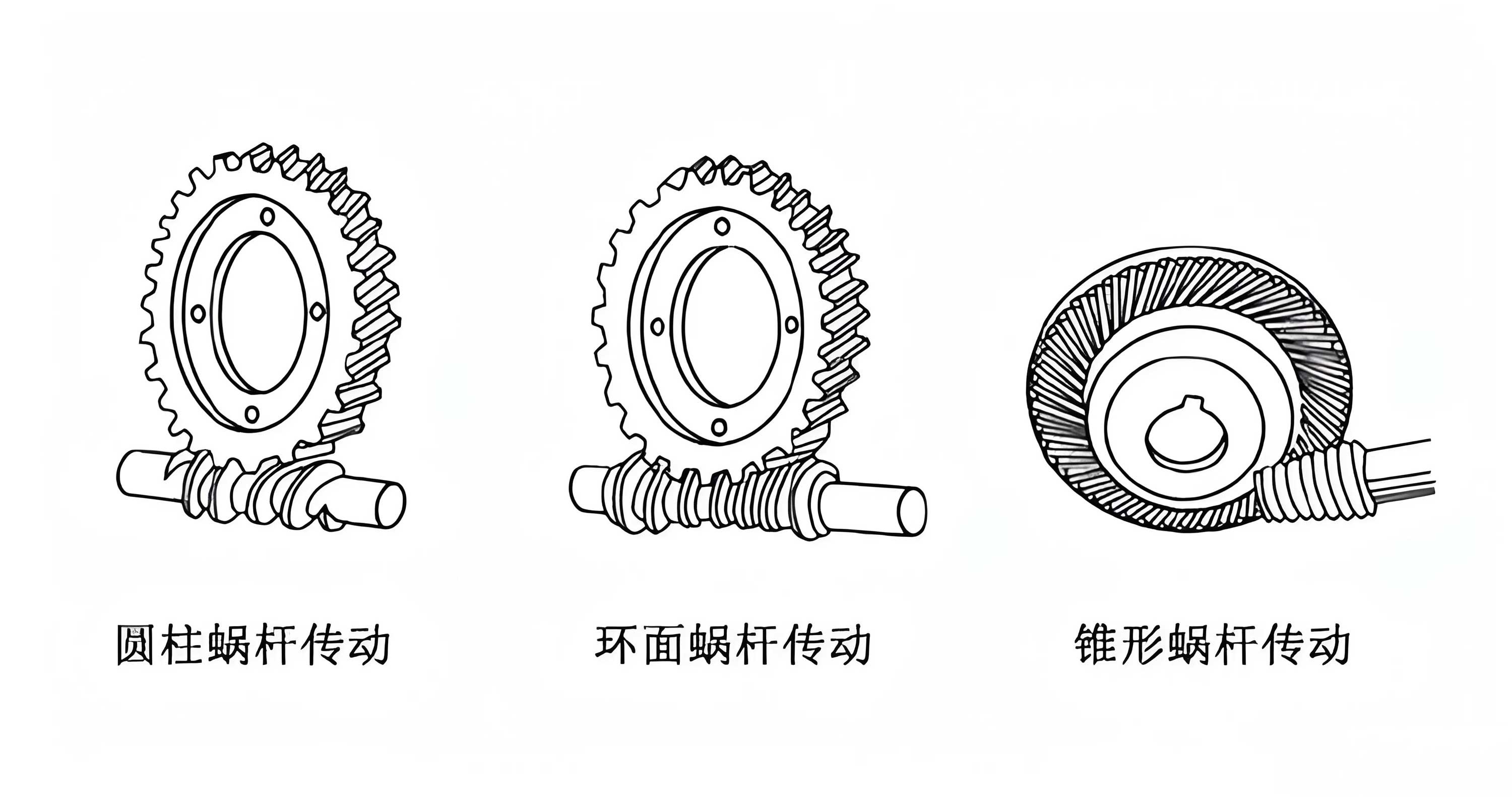
A worm gear set consists of a screw-like worm meshing with a toothed gear, the worm wheel. This configuration offers distinct benefits, including very high single-stage reduction ratios, compact and space-saving design, smooth and quiet operation due to the sliding contact, and the potential for self-locking, which prevents back-driving. However, these advantages are accompanied by a significant drawback: the sliding action between the worm and wheel teeth inherently generates substantial friction, leading to lower transmission efficiency compared to gear pairs with primarily rolling contact. To mitigate this frictional wear, the worm wheel is typically manufactured from costly, high-strength, and wear-resistant non-ferrous materials, such as tin bronze. Consequently, a primary objective in the economical design of worm gears becomes the minimization of the volume of this expensive material required for the wheel’s working ring. By optimizing the design parameters, we can achieve a more compact, lighter, and crucially, a more cost-effective worm gear assembly without compromising its functional performance or longevity.
Mathematical Model for Worm Gears Optimization
The foundation of any systematic optimization process is a well-defined mathematical model. This model encapsulates the design goal as an objective function, identifies the parameters we can adjust as design variables, and establishes the limits of their adjustment through a set of constraints derived from physical laws, material properties, and design standards.
Objective Function: Minimizing Material Volume
The core objective is to minimize the volume of the non-ferrous metal ring of the worm wheel. The volume of this annular ring can be calculated from its basic dimensions: outer diameter ($$d_e$$), inner diameter ($$d_0$$), and face width ($$b$$).
$$ V = \frac{\pi b}{4} (d_e^2 – d_0^2) $$
For standard cylindrical worm gears, these dimensions are expressed in terms of fundamental design parameters. The outer diameter coefficient ($$\psi_e$$) and face width coefficient ($$\psi_b$$) are typically chosen based on empirical design practice; common values are $$\psi_e = 1.5$$ and $$\psi_b = 0.75$$. The inner diameter is related to the root diameter. Incorporating standard geometrical relationships for worm gears, the volume can be reformulated as a function of the module ($$m$$), the number of worm threads ($$z_1$$), the diameter factor or quotient ($$q = d_1 / m$$, where $$d_1$$ is the worm reference diameter), and the gear ratio ($$i$$).
$$ V = \frac{\pi \psi_b (q+2) m^3}{4} \left[ (i z_1 + \psi_e + 2)^2 – (i z_1 – 4.4)^2 \right] $$
This equation forms our primary objective function. The goal of the optimization is to find the combination of $$z_1$$, $$m$$, and $$q$$ that yields the smallest possible value for $$V$$.
Design Variables and Simplified Objective
From the volume equation, it is clear that the volume of the worm wheel’s ring depends on the number of worm threads ($$z_1$$), the module ($$m$$), and the diameter quotient ($$q$$). The gear ratio ($$i$$) is usually a predetermined requirement from the application. Therefore, we define our design variable vector as:
$$ \mathbf{x} = (x_1, x_2, x_3)^T = (z_1, m, q)^T $$
Substituting the standard values for the coefficients ($$\psi_b=0.75$$, $$\psi_e=1.5$$) and simplifying the algebraic expression, the objective function can be written in a more compact form suitable for computational optimization:
$$ f(\mathbf{x}) = 1.48 \pi (x_3 + 2) (2 i x_1 – 0.9) x_2^3 $$
Where $$f(\mathbf{x})$$ represents the volume $$V$$ to be minimized.
Constraint Conditions
The design variables cannot be chosen arbitrarily. They must satisfy a series of constraints that ensure the worm gear set will function reliably under the specified operating conditions. These constraints are categorized into performance constraints and boundary constraints.
Performance Constraints
These are derived from the fundamental failure modes and operational limits of worm gears.
1. Contact Stress Constraint: The primary failure mode for worm gears is surface pitting due to excessive contact (Hertzian) stress at the tooth interface. The contact stress must be below the allowable stress ($$[\sigma_H]$$) of the wheel material. The standard contact strength condition is formulated as:
$$ m \sqrt[3]{q} \ge \sqrt[3]{\frac{K T_2}{15150 \cdot \frac{z_2}{i} [\sigma_H]^2}} $$
Where:
- $$K$$ is the load factor,
- $$T_2$$ is the torque on the worm wheel, calculated from input power ($$P_1$$) and speed ($$n_1$$): $$T_2 = 9550 \cdot i \cdot \eta \cdot P_1 / n_1$$,
- $$\eta$$ is the approximate efficiency: $$\eta \approx 1 – 0.035\sqrt{i}$$,
- $$z_2 = i \cdot z_1$$ is the number of teeth on the worm wheel.
Rearranging this inequality to the standard form $$g(\mathbf{x}) \le 0$$ gives the first performance constraint:
$$ g_1(\mathbf{x}) = \left( \frac{K T_2}{15150 \cdot x_1 [\sigma_H]^2} \right)^{2/3} – x_2 \sqrt[3]{x_3} \le 0 $$
A more computationally direct form used in the algorithm is:
$$ g_1(\mathbf{x}) = \frac{K T_2}{(15150 \cdot i \cdot x_1 \cdot [\sigma_H])^2} – x_2^3 \cdot x_3 \le 0 $$
2. Worm Shaft Deflection Constraint: Excessive deflection of the worm shaft can lead to poor tooth engagement, localized loading, and increased wear. The maximum deflection ($$y$$) at the midpoint of the shaft must be limited to a fraction of the worm pitch diameter (typically $$0.001 d_1$$). The deflection is calculated from beam theory under combined radial and tangential loads:
$$ y = \frac{\sqrt{F_{t1}^2 + F_{r1}^2} \cdot L^3}{48 E J} \le 0.001 d_1 = 0.001 m q $$
Where:
- $$F_{t1} = 2T_1 / (m q)$$ is the tangential force on the worm,
- $$F_{r1} \approx (2T_2 \tan 20^\circ) / (i z_1 m)$$ is the radial force,
- $$L \approx 0.9 \cdot m \cdot i \cdot z_1$$ is the approximate span between supports,
- $$E$$ is the modulus of elasticity (for steel),
- $$J = \pi m^4 (q – 2.4)^4 / 64$$ is the second moment of area of the worm’s root section.
Substituting these expressions and rearranging yields the second performance constraint:
$$ g_2(\mathbf{x}) = 0.729 i^3 x_1^3 \sqrt{ \left( \frac{2T_1}{x_2 x_3} \right)^2 + \left( \frac{2T_2 \tan(\pi/9)}{i x_1 x_2} \right)^2 } – 157.7 \pi x_2^2 x_3 (x_3 – 2.4)^4 \le 0 $$
Boundary Constraints
These constraints define the practical and standardized ranges for the design variables based on common design practice for medium-power drives.
| Variable | Description | Lower Bound | Upper Bound | Constraint Inequality |
|---|---|---|---|---|
| $$x_1$$ | Number of worm threads, $$z_1$$ | 2 | 3 | $$g_3(\mathbf{x})=2 – x_1 \le 0$$ $$g_4(\mathbf{x})=x_1 – 3 \le 0$$ |
| $$x_2$$ | Module, $$m$$ (mm) | 3 | 5 | $$g_5(\mathbf{x})=3 – x_2 \le 0$$ $$g_6(\mathbf{x})=x_2 – 5 \le 0$$ |
| $$x_3$$ | Diameter quotient, $$q$$ | 5 | 16 | $$g_7(\mathbf{x})=5 – x_3 \le 0$$ $$g_8(\mathbf{x})=x_3 – 16 \le 0$$ |
Thus, the complete optimization problem for these worm gears is formally stated as:
Find the vector $$\mathbf{x} = (z_1, m, q)^T$$
that minimizes $$f(\mathbf{x}) = 1.48 \pi (q + 2) (2 i z_1 – 0.9) m^3$$
subject to the constraints $$g_j(\mathbf{x}) \le 0, \quad j = 1, 2, …, 8$$.
Fundamentals of the Genetic Algorithm (GA)
To solve this constrained, nonlinear optimization problem, we employ a Genetic Algorithm (GA). GAs are population-based metaheuristic optimization techniques inspired by the principles of natural selection and genetics. Unlike traditional gradient-based methods that may converge to a local optimum, GAs are renowned for their strong global search capabilities, implicit parallelism, and robustness when dealing with complex, discontinuous, or multi-modal objective functions. This makes them particularly suitable for engineering design problems like the optimization of worm gears, where the design space may have several local minima.
The GA operates on a population of potential solutions, called individuals or chromosomes. Each chromosome is a string (often binary or real-valued) encoding the values of the design variables. The algorithm progresses through generations, applying genetic operators to evolve the population towards better regions of the search space. The main steps in a standard GA are:
- Initialization: A first population of random chromosomes is generated within the specified variable bounds.
- Fitness Evaluation: Each chromosome is decoded into a design vector $$\mathbf{x}$$. Its performance is evaluated using a fitness function. For a minimization problem like ours, a lower objective function value (volume) should correspond to higher fitness. Crucially, the fitness function must also account for constraint violation.
- Selection: Chromosomes are selected for reproduction based on their fitness. Fit individuals have a higher probability of being selected, mimicking “survival of the fittest.” Common methods include roulette wheel selection and tournament selection.
- Crossover: Pairs of selected parent chromosomes exchange genetic information to produce offspring, exploring new combinations of design parameters.
- Mutation: Random alterations are introduced into the offspring’s chromosome with a small probability. This operator helps maintain population diversity and enables the exploration of new areas in the search space, preventing premature convergence.
- Termination: The process repeats (evaluation, selection, crossover, mutation) until a termination criterion is met, such as reaching a maximum number of generations, finding a satisfactory solution, or observing convergence of the population.
Constructing the Fitness Function for Constrained Optimization
A critical step in applying GA to engineering problems is designing an appropriate fitness function. For constrained optimization, a common and effective approach is the penalty function method. The idea is to transform the constrained problem into an unconstrained one by adding a penalty term to the objective function whenever constraints are violated.
We define a fitness function $$\text{Val}(\mathbf{x})$$ for our minimization problem as follows:
$$ \text{Val}(\mathbf{x}) = f(\mathbf{x}) + P(\mathbf{x}) $$
Here, $$P(\mathbf{x})$$ is the penalty term. Using an exterior penalty method, the penalty is zero for feasible designs and positive for infeasible ones. A quadratic penalty is often used:
$$ P(\mathbf{x}) = \begin{cases}
0, & \text{if } \mathbf{x} \text{ is feasible (all } g_j(\mathbf{x}) \le 0\text{)} \\
\sum_{j=1}^{m} r_j \cdot [\max(0, g_j(\mathbf{x}))]^2, & \text{otherwise}
\end{cases} $$
Where $$r_j$$ are positive penalty coefficients. Since our constraints are already in the form $$g_j(\mathbf{x}) \le 0$$, the term $$\max(0, g_j(\mathbf{x}))$$ is simply $$g_j(\mathbf{x})$$ when it is positive (violated). The fitness value to be minimized by the GA is therefore $$\text{Val}(\mathbf{x})$$. In practice, because many GA implementations are designed to maximize fitness, the mapping is often inverted, e.g., $$\text{Fitness}(\mathbf{x}) = -\text{Val}(\mathbf{x})$$.
Implementation of GA for Worm Gears Optimization in MATLAB
MATLAB provides a powerful environment for implementing this optimization strategy, either through programming a custom GA or using its Global Optimization Toolbox. The process typically involves the following steps, which we apply to our specific case of worm gears optimization.
Problem Specification and Parameters
First, we define the fixed operating conditions and material properties for our example worm gear drive:
| Parameter | Symbol | Value | Unit |
|---|---|---|---|
| Input Power | $$P_1$$ | 6 | kW |
| Input Speed | $$n_1$$ | 1450 | rpm |
| Gear Ratio | $$i$$ | 20 | – |
| Load Factor | $$K$$ | 1.1 | – |
| Allowable Contact Stress | $$[\sigma_H]$$ | 220 | MPa |
| Worm Material | – | Steel (20CrMnTi) | – |
| Wheel Material | – | Tin Bronze (ZCuSn10Pb1) | – |
From these, we calculate the derived constants: efficiency $$\eta$$, input torque $$T_1$$, and output torque $$T_2$$.
Fitness Function Definition
A MATLAB function file (e.g., `fitnessFunction.m`) is created to compute the fitness (or penalty-based objective) for any given design vector `x = [z1, m, q]`. The core of this function is structured as follows:
(Pseudo-code representation)
function fitnessValue = fitnessFunction(x)
% Unpack variables
z1 = x(1); m = x(2); q = x(3);
% Fixed parameters (i, P1, n1, K, sigma_HP)
…
% 1. Calculate objective (volume)
V = 1.48 * pi * (q+2) * (2*i*z1 – 0.9) * m^3;
% 2. Calculate constraint violations
g1 = … % Contact stress constraint
g2 = … % Deflection constraint
% 3. Apply penalty coefficients (e.g., r0=0.1, r1=0.05)
penalty = 0;
if g1 > 0, penalty = penalty + 0.1 * g1^2; end
if g2 > 0, penalty = penalty + 0.05 * g2^2; end
% 4. Total value to minimize
totalValue = V + penalty;
% 5. Return negative for GA maximization
fitnessValue = -totalValue;
end
GA Configuration and Execution
Using MATLAB’s `ga` optimizer, we configure the algorithm parameters. The success of optimizing worm gears depends significantly on appropriate GA settings:
| GA Parameter | Typical Setting / Choice | Rationale |
|---|---|---|
| Population Size | 50 – 100 | Balances exploration capability and computational cost. |
| Creation Function | `’gacreationuniform’` or custom bounds | Ensures initial population is within variable bounds. |
| Fitness Scaling | `’fitscalingrank’` | Helps prevent premature convergence by reducing early dominance of super-individuals. |
| Selection Function | `’selectiontournament’` (size 2-4) | Tournament selection provides good selective pressure. |
| Crossover Function | `’crossoverintermediate’` (ratio ~0.8) | Creates offspring as weighted averages of parents, suitable for real-valued genes. |
| Mutation Function | `’mutationadaptfeasible’` | Adaptively mutates within bounds, respecting linear constraints. |
| Crossover Fraction | 0.8 | 80% of next generation from crossover. |
| Stopping Criterion | `’MaxGenerations’, 500` or Stall Generations | Allows sufficient evolution; stall check stops if no improvement. |
The optimization is executed with a command similar to:
`[x_opt, fval] = ga(@fitnessFunction, 3, [], [], [], [], [2;3;5], [3;5;16], [], options);`
Where the lower bounds are `[2;3;5]` and upper bounds are `[3;5;16]` for `[z1; m; q]`.
Analysis of Optimization Results for Worm Gears
Running the GA for the specified problem typically yields convergence within a few hundred generations. The algorithm finds an optimal point in the continuous design space. For instance, a stable solution might be:
$$ z_1^* = 2.9969, \quad m^* = 3.9910 \, \text{mm}, \quad q^* = 15.2265 $$
$$ V_{\text{min}} = 605,794.2 \, \text{mm}^3 $$
Engineering design requires standard, manufacturable values. Therefore, we round these optimal continuous variables to the nearest preferred or standard values:
$$ z_1 = 3, \quad m = 4 \, \text{mm}, \quad q = 16 $$
Substituting these rounded values back into the volume equation gives the final, practical optimum volume. We then must verify that this rounded design still satisfies all performance constraints, which it typically does as the continuous optimum lies within the feasible region.
The effectiveness of the optimization for these worm gears is best illustrated by comparing the GA-optimized design with a conventional design derived from standard handbook procedures or iterative trial-and-error.
| Design Item | Conventional Design | GA-Optimized Design (Rounded) | Improvement |
|---|---|---|---|
| Number of Worm Threads ($$z_1$$) | 2 | 3 | +50% (leads to smaller wheel) |
| Module, $$m$$ (mm) | 5 | 4 | -20% |
| Diameter Quotient, $$q$$ | 18 | 16 | -11.1% |
| Worm Reference Diameter, $$d_1=mq$$ (mm) | 90 | 64 | -28.9% |
| Wheel Ring Volume, $$V$$ (mm³) | 920,226.5 | 637,934.1 | -30.7% |
The results are striking. The genetic algorithm for worm gears optimization converged to a solution that uses a 3-thread worm instead of the more common 1 or 2-thread design for high ratios. This increases the lead angle, which generally improves efficiency and, as shown, significantly reduces the required size of the mating worm wheel. Coupled with a reduction in both module and diameter quotient, the overall material volume for the bronze ring is reduced by over 30%. This translates directly to substantial cost savings in material and a more compact, lighter gearbox assembly.
Discussion and Further Considerations
The successful application of the Genetic Algorithm to the worm gears optimization problem demonstrates its power as a global search tool. Unlike local search methods that might get trapped by the initial guess, the GA explores the design space broadly. The penalty function method effectively guides the search towards the feasible region while minimizing the objective. The choice of penalty coefficients ($$r_j$$) is important; too small a penalty may allow infeasible but low-volume solutions to dominate, while too large a penalty may hinder exploration near constraint boundaries. Adaptive penalty schemes can be implemented for more challenging problems.
The model presented here can be extended and refined in several ways to create an even more comprehensive tool for the optimal design of worm gears:
- Additional Constraints: While bending strength is often secondary in worm wheels, it can be included for completeness. Thermal constraints are critical for worm gears due to their lower efficiency; a constraint limiting the operating temperature or requiring a specific heat dissipation capacity could be added to ensure thermal stability.
- Multi-Objective Optimization: The current model is single-objective (minimize volume). In practice, designers may wish to simultaneously maximize efficiency ($$\eta$$) or minimize center distance. This transforms the problem into a multi-objective one, which can be solved using algorithms like NSGA-II (Non-dominated Sorting Genetic Algorithm II), producing a set of Pareto-optimal solutions representing trade-offs between competing goals.
- Refined Modeling: The approximate formula for efficiency ($$\eta \approx 1 – 0.035\sqrt{i}$$) and other simplifications can be replaced with more precise analytical or empirical models based on the specific tooth geometry (ZA, ZN, ZI, ZK types) and lubrication conditions.
- Manufacturing and Standardization Constraints: The algorithm can be modified to favor solutions where the module and worm diameters align with standard, readily available tooling and bearing sizes, further enhancing practical applicability.
Conclusion
In this detailed exploration, we have established a complete framework for the optimization of worm gears design using a Genetic Algorithm. The process begins with formulating a precise mathematical model where the volume of the worm wheel’s bronze ring is the objective function to be minimized, subject to essential constraints concerning contact strength, shaft deflection, and practical design limits. The Genetic Algorithm, with its inherent global search capabilities and robustness, is then employed to solve this constrained nonlinear optimization problem. Implementation in MATLAB provides a flexible and powerful platform for this task.
The results unequivocally demonstrate the significant benefits of applying such a systematic optimization approach to the design of worm gears. Compared to a conventional design methodology, the GA-optimized solution achieved a reduction in material volume exceeding 30%. This optimization leads directly to lower material costs, reduced weight, and a more compact transmission layout. Furthermore, the process is automated and reproducible, reducing reliance on designer experience and trial-and-error. While the presented model is a robust starting point, it lays the groundwork for future enhancements, such as multi-objective optimization and more sophisticated physical constraints. In conclusion, the integration of Genetic Algorithms into the design process represents a highly effective and valuable methodology for advancing the performance and economy of worm gear drives.