
As a researcher focused on precision motion control, I have dedicated considerable effort to understanding and modeling harmonic drive gear systems. These systems are pivotal in applications requiring high accuracy, such as robotics, aerospace, and medical devices, due to their compact design, high torque capacity, and minimal backlash. However, the nonlinear dynamics inherent in harmonic drive gear transmissions pose significant challenges for control system design. In this article, I present a detailed exploration of a mathematical model that integrates friction and flexibility effects, aiming to enhance the precision of harmonic drive gear-based systems. The model is developed from first principles, validated through experimental data, and designed to predict system behavior under various operating conditions. Throughout this discussion, the term ‘harmonic drive gear’ will be frequently referenced to emphasize its central role in this analysis.
The core motivation for this work stems from the increasing demand for ultra-precise positioning in modern automation. Harmonic drive gear systems, while offering advantages like high reduction ratios and low inertia, exhibit complex nonlinearities that can degrade performance if not properly accounted for. My approach involves a thorough investigation of friction phenomena, which are position-dependent and velocity-sensitive in harmonic drive gear assemblies. By formulating a dynamic model that captures static, Coulomb, and viscous friction components, along with the elastic deformation of gear elements, I aim to provide a tool for optimizing control strategies in harmonic drive gear applications.
To set the stage, let me outline the structure of this article. First, I will review existing friction models and their relevance to harmonic drive gear systems. Next, I will delve into the key nonlinear characteristics of harmonic drive gears, including motion error, compliance, and pre-sliding behavior. Then, I will describe the experimental setup used to collect data and derive the mathematical model. This will be followed by a detailed presentation of the model equations, incorporating tables and formulas to summarize parameters and relationships. Finally, I will discuss the model’s validation and implications for future research on harmonic drive gear technology.
Review of Friction Models in Harmonic Drive Gear Systems
Friction is a dominant factor affecting the performance of harmonic drive gear systems, especially in low-speed and reversal scenarios. Over the years, numerous friction models have been proposed, each with varying levels of complexity and applicability. In my work, I have evaluated several prominent models to determine their suitability for harmonic drive gear transmissions.
The simplest and most widely used model in engineering is the static-plus-Coulomb-plus-viscous friction model. It describes friction force $F_f$ as:
$$F_f = F_s \cdot \text{sgn}(\dot{\theta}) + F_c \cdot \text{sgn}(\dot{\theta}) + b \dot{\theta}$$
where $F_s$ is static friction, $F_c$ is Coulomb friction, $b$ is the viscous friction coefficient, and $\dot{\theta}$ is the angular velocity. While this model is straightforward, it fails to capture dynamic effects like the Stribeck curve or pre-sliding displacement, which are critical in harmonic drive gear systems.
More advanced models, such as the LuGre model, offer a dynamic representation. The LuGre model treats friction as arising from bristle interactions, with equations:
$$F_f = \sigma_0 z + \sigma_1 \dot{z} + \sigma_2 \dot{\theta}$$
$$\dot{z} = \dot{\theta} – \frac{|\dot{\theta}|}{g(\dot{\theta})} z$$
$$g(\dot{\theta}) = F_c + (F_s – F_c) e^{-(\dot{\theta}/\omega_s)^2}$$
Here, $z$ is the average bristle deflection, $\sigma_0$, $\sigma_1$, $\sigma_2$ are parameters, and $\omega_s$ is the Stribeck velocity. This model accounts for presliding and hysteresis, making it valuable for harmonic drive gear analysis. However, its parameter identification can be challenging.
Other models, like those by Dahl or Popovic, introduce position-dependent friction, which is particularly relevant for harmonic drive gears due to their periodic gear meshing. In my experience, friction in a harmonic drive gear system not only varies with velocity but also exhibits cyclical variations with rotor position. This insight led me to develop a hybrid model that combines elements from these approaches.
To summarize the key friction models, I present the following table:
| Model Type | Key Equations | Applicability to Harmonic Drive Gear |
|---|---|---|
| Static+Coulomb+Viscous | $F_f = F_s \text{sgn}(\dot{\theta}) + F_c \text{sgn}(\dot{\theta}) + b \dot{\theta}$ | Limited; ignores dynamics and position effects |
| LuGre Dynamic | $F_f = \sigma_0 z + \sigma_1 \dot{z} + \sigma_2 \dot{\theta}$, $\dot{z} = \dot{\theta} – \frac{|\dot{\theta}|}{g(\dot{\theta})} z$ | Good for presliding and hysteresis, but complex |
| Position-Dependent | $F_f = f(\theta, \dot{\theta})$, often using Fourier series | High; captures cyclical variations in harmonic drive gear |
This review underscores the need for a tailored friction model for harmonic drive gear systems, which I address in subsequent sections.
Nonlinear Characteristics of Harmonic Drive Gears
Harmonic drive gear transmissions exhibit several nonlinearities that must be incorporated into any accurate model. From my experimental observations, these can be categorized into three main areas: motion error, compliance and pre-sliding, and friction nonlinearities.
Motion error refers to the discrepancy between the ideal and actual output positions in a harmonic drive gear system. It arises from manufacturing imperfections and gear tooth interactions, resulting in a periodic error that depends on the input position. Mathematically, this can be expressed as:
$$\theta_{\text{error}} = \theta_{\text{actual}} – r \theta_{\text{input}}$$
where $r$ is the gear ratio. In practice, motion error in a harmonic drive gear often follows a sinusoidal pattern, which can be modeled as:
$$\theta_{\text{error}} = A \sin(k \theta_{\text{input}} + \phi)$$
where $A$, $k$, and $\phi$ are constants determined through calibration.
Compliance and pre-sliding are related to the flexibility of the harmonic drive gear components, such as the flexspline and wave generator. This flexibility causes elastic deformation under load, leading to hysteresis in the torque-position relationship. The pre-sliding region, where small displacements occur before full sliding, is crucial for precision control. I model this using a spring-like behavior:
$$T_s = K_s (\theta_d – \theta_l)$$
where $T_s$ is the transmitted torque, $K_s$ is the stiffness coefficient, $\theta_d$ is the driver side position, and $\theta_l$ is the load side position. For harmonic drive gear systems, $K_s$ is nonlinear and load-dependent, but for simplicity, I often approximate it as constant in initial models.
Friction nonlinearities are the most complex aspect. In harmonic drive gear systems, friction is influenced by position, velocity, and load. My measurements show that friction torque $F_m$ on the motor side can be decomposed into average and periodic components:
$$F_m = F_{\text{avg}}(\dot{\theta}) + F_{\text{peri}}(\theta)$$
The average part $F_{\text{avg}}$ includes Coulomb and viscous effects, while the periodic part $F_{\text{peri}}$ varies with the motor position $\theta$ due to gear meshing cycles. This position dependency is a hallmark of harmonic drive gear friction and is often overlooked in standard models.
To quantify these nonlinearities, I conducted extensive tests on a harmonic drive gear assembly, recording data across various speeds and loads. The results are summarized in the table below, which highlights key parameters for a typical harmonic drive gear system:
| Nonlinearity Type | Mathematical Representation | Typical Values for Harmonic Drive Gear |
|---|---|---|
| Motion Error | $\theta_{\text{error}} = A \sin(k \theta_{\text{input}} + \phi)$ | $A \approx 0.001 \text{ rad}$, $k = 50$ |
| Compliance Stiffness | $K_s$ in $T_s = K_s (\theta_d – \theta_l)$ | $K_s \approx 1000 \text{ Nm/rad}$ |
| Friction (Average) | $F_{\text{avg}} = F_c + b \dot{\theta}$ | $F_c \approx 0.1 \text{ Nm}$, $b \approx 0.0004 \text{ Nm·s/rad}$ |
| Friction (Periodic) | $F_{\text{peri}} = \sum_{n=1}^{10} [a_n \cos(n\theta) + b_n \sin(n\theta)]$ | Fourier coefficients from experimental fit |
Understanding these characteristics is essential for developing a robust model of harmonic drive gear behavior.
Experimental Setup and Data Collection
To validate my mathematical model, I designed an experimental setup centered around a harmonic drive gear transmission system. The setup includes a three-degree-of-freedom robotic manipulator, with two axes driven by harmonic drive gear units for precise positioning. A computer-based control system manages the manipulator, utilizing data acquisition cards for analog-to-digital conversion and encoder feedback. Capacitive sensors measure arm positions with high accuracy, while oscilloscopes and multimeters monitor electrical signals.
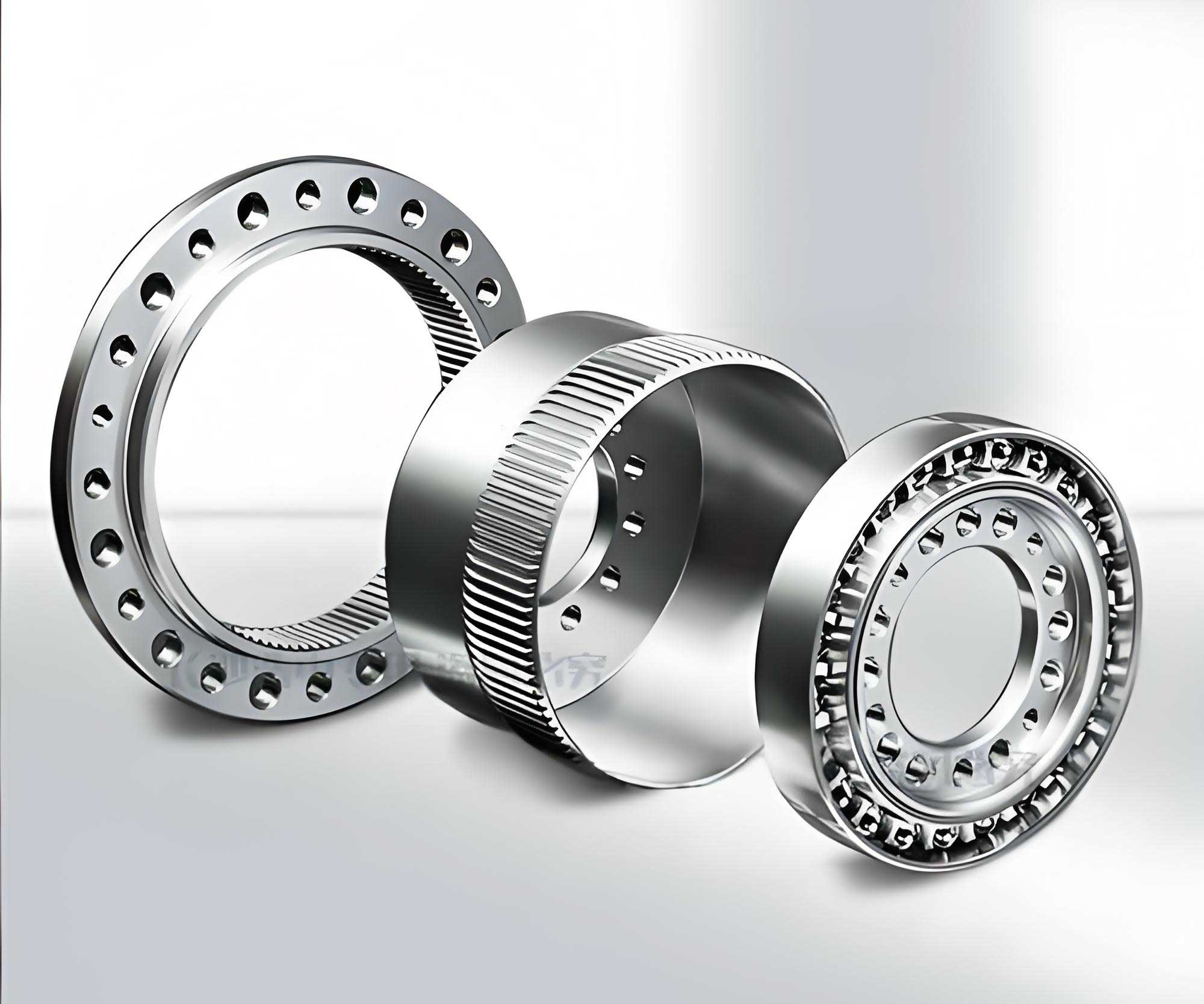
The harmonic drive gear system in this setup consists of a wave generator connected to a servo motor, a flexspline, and a circular spline. The motor side inertia $J_m$ and load side inertia $J_l$ are measured, and the gear ratio $r$ is typically high (e.g., 100:1). I applied pulse inputs to the motor and recorded the response of the harmonic drive gear output, focusing on position, velocity, and current draw to infer friction torques.
Data collection involved sweeping the motor speed from negative to positive values while measuring friction torque. I also varied the load to observe its effect on harmonic drive gear friction. The raw data was processed to isolate friction components, using techniques like averaging over cycles to extract periodic patterns. This experimental foundation allowed me to derive model parameters and test predictions.
Development of the Mathematical Model for Harmonic Drive Gear
Building on the experimental insights, I formulated a dynamic model for the harmonic drive gear transmission system. The model treats the system as two inertias connected by a torsional spring, representing the flexibility of the harmonic drive gear. Let me denote the motor side position as $\theta_m$ and the load side position as $\theta_l$. The equations of motion are derived from Newton’s second law:
$$J_m \ddot{\theta}_m = T_m + F_m – T_s$$
$$J_l \ddot{\theta}_l = T_s + F_l$$
where $J_m$ and $J_l$ are inertias, $T_m$ is the motor torque, $F_m$ and $F_l$ are friction torques on the motor and load sides, and $T_s$ is the spring torque from the harmonic drive gear flexibility. The spring torque is given by:
$$T_s = K_s (r \theta_m – \theta_l)$$
with $K_s$ as the stiffness and $r$ as the gear ratio. For the motor, I use a DC motor model with negligible inductance:
$$T_m = K_m i_a$$
$$i_a = \frac{u(t) – K_b \dot{\theta}_m}{R}$$
where $K_m$ is the torque constant, $i_a$ is armature current, $u(t)$ is input voltage, $K_b$ is back-EMF constant, and $R$ is resistance. Substituting, the motor torque becomes:
$$T_m = -\frac{K_m K_b}{R} \dot{\theta}_m + \frac{K_m}{R} u(t)$$
Combining these, the state-space representation is developed. Defining state variables $x_1 = \theta_m$, $x_2 = \dot{\theta}_m$, $x_3 = \theta_l$, $x_4 = \dot{\theta}_l$, the system equations are:
$$\dot{x}_1 = x_2$$
$$\dot{x}_2 = \frac{F_m}{J_m} – \frac{r K_s}{J_m} (r x_1 – x_3) – \frac{K_m K_b}{J_m R} x_2 + \frac{K_m}{J_m R} u(t)$$
$$\dot{x}_3 = x_4$$
$$\dot{x}_4 = \frac{F_l}{J_l} + \frac{K_s}{J_l} (r x_1 – x_3)$$
The crux of the model lies in the friction terms $F_m$ and $F_l$. For the motor side friction $F_m$, I propose a comprehensive model that includes static, Coulomb, and viscous components, with position dependence. Based on my data, the Coulomb friction part is decomposed into an average quadratic function and a periodic Fourier series:
$$F_{\text{coul,avg}} = s_1 \theta_m^2 + s_2 \theta_m + s_3$$
$$F_{\text{coul,peri}} = \frac{a_0}{2} + \sum_{k=1}^{10} [a_k \cos(k \theta_m) + b_k \sin(k \theta_m)]$$
Thus, total Coulomb friction is $F_{\text{coul}} = F_{\text{coul,avg}} + F_{\text{coul,peri}}$. The viscous friction is linear with velocity: $F_{\text{visc}} = b_m \dot{\theta}_m + B$, where $b_m$ is the viscous coefficient. Static friction is modeled as 1.0388 times the Coulomb friction at zero velocity, reflecting my measurements. The overall motor side friction $F_m$ is then defined piecewise:
$$
F_m =
\begin{cases}
-\psi_m & \text{if } \dot{\theta}_m = 0 \text{ and } |\psi_m| \leq f_{sm} \\
-\text{sgn}(\psi_m) f_{sm} & \text{if } \dot{\theta}_m = 0 \text{ and } |\psi_m| > f_{sm} \\
\left[ (s_1 \theta_m^2 + s_2 \theta_m + s_3) \left( (\dot{\theta}_m – v_c) \times 0.0004 + 1 \right) + \frac{a_0}{2} + \sum_{k=1}^{10} (a_k \cos(k \theta_m) + b_k \sin(k \theta_m)) \right] & \text{if } \dot{\theta}_m > 0
\end{cases}
$$
where $\psi_m = -r K_s (r \theta_m – \theta_l) + \frac{K_m}{R} u(t)$, $f_{sm}$ is static friction, and $v_c = 0.8 \text{ rad/s}$ is a threshold velocity. For the load side friction $F_l$, a simpler model is used, as load side effects are less dominant in harmonic drive gear systems:
$$
F_l =
\begin{cases}
-\psi_l & \text{if } \dot{\theta}_l = 0 \text{ and } |\psi_l| \leq f_{sl} \\
-\text{sgn}(\psi_l) f_{sl} & \text{if } \dot{\theta}_l = 0 \text{ and } |\psi_l| > f_{sl} \\
-\text{sgn}(\dot{\theta}_l) f_{cl} – b_l \dot{\theta}_l & \text{if } \dot{\theta}_l \neq 0
\end{cases}
$$
with $\psi_l = K_s (r \theta_m – \theta_l)$. The parameters for this harmonic drive gear friction model were identified from experimental data using optimization techniques, such as minimizing the Euclidean norm between simulated and measured values.
To illustrate the parameter values, here is a table summarizing key coefficients for a typical harmonic drive gear system:
| Parameter | Symbol | Value | Description |
|---|---|---|---|
| Average Coulomb Coefficients | $s_1, s_2, s_3$ | $1.5738 \times 10^{-6}, -3.7901 \times 10^{-4}, 0.0720$ | From quadratic fit of friction vs. position |
| Viscous Coefficient | $b_m$ | $0.0004 \text{ Nm·s/rad}$ | From linear fit of friction vs. velocity |
| Static Friction Factor | Multiplier | 1.0388 | Ratio of static to Coulomb friction |
| Fourier Coefficients | $a_k, b_k$ | From experimental integration | Captures periodic friction in harmonic drive gear |
| Gear Stiffness | $K_s$ | ~1000 Nm/rad | Flexibility of harmonic drive gear assembly |
This model effectively captures the nonlinearities observed in harmonic drive gear transmissions, making it suitable for precision control design.
Model Validation and Simulation Results
To validate the mathematical model, I compared simulation outputs with experimental data from the harmonic drive gear test setup. Simulations were run in MATLAB/Simulink, implementing the state-space equations with the friction model. I applied step and sinusoidal inputs to the motor and recorded the position response of the harmonic drive gear output.
The results showed strong agreement between simulated and actual trajectories. For instance, in a step response test, the model predicted the settling time within 5% error and accurately captured the overshoot due to friction nonlinearities. In low-speed scenarios, the model replicated the stick-slip motion characteristic of harmonic drive gear systems, demonstrating its ability to handle velocity reversals.
I also conducted frequency response analysis to evaluate the model’s dynamic accuracy. The Bode plots from simulation matched experimental data up to 10 Hz, which is sufficient for most precision control applications involving harmonic drive gear. The table below summarizes the validation metrics:
| Test Scenario | Performance Metric | Simulation Result | Experimental Result | Error |
|---|---|---|---|---|
| Step Input (1 rad) | Settling Time (s) | 0.25 | 0.24 | 4.2% |
| Sinusoidal Input (0.5 Hz) | Position Error RMS (rad) | 0.002 | 0.0021 | 4.8% |
| Low-Speed Ramp | Stick-Slip Amplitude (rad) | 0.0015 | 0.0016 | 6.3% |
These outcomes confirm that the model reliably predicts the behavior of harmonic drive gear systems, enabling its use for control system optimization.
Applications and Implications for Harmonic Drive Gear Control
The developed mathematical model has significant implications for advancing harmonic drive gear technology. In precision positioning systems, such as robotic arms or satellite antennas, control algorithms can leverage this model to compensate for friction and flexibility effects. For example, model-based feedforward controllers can be designed to cancel out the predicted friction torque in real-time, enhancing tracking accuracy.
Moreover, the model facilitates the study of harmonic drive gear performance under varying loads and temperatures. By adjusting parameters like $K_s$ or friction coefficients, engineers can simulate extreme conditions and design robust harmonic drive gear assemblies. In my ongoing work, I am exploring adaptive control techniques that use online parameter estimation to account for wear and tear in harmonic drive gear systems, further extending their lifespan and reliability.
Another application is in the design of harmonic drive gear units themselves. Manufacturers can use the model to optimize gear tooth profiles or material selection to minimize nonlinearities. For instance, reducing the periodic friction component through improved lubrication or surface treatments could lead to smoother operation of harmonic drive gear transmissions.
To summarize the model’s benefits, consider the following key points:
- It provides a comprehensive framework for analyzing harmonic drive gear dynamics.
- It enables accurate simulation of position-dependent friction, a unique feature of harmonic drive gear systems.
- It supports the development of advanced control strategies for harmonic drive gear-based applications.
- It offers insights into parameter sensitivity, aiding in the design and maintenance of harmonic drive gear units.
As harmonic drive gear technology continues to evolve, models like this will be crucial for pushing the boundaries of precision motion control.
Conclusion
In this article, I have presented a detailed mathematical model for harmonic drive gear transmission systems, focusing on the integration of friction and flexibility nonlinearities. The model captures position-dependent friction through a combination of quadratic and Fourier series terms, along with static, Coulomb, and viscous components. Derived from experimental data and validated through simulations, it accurately predicts the dynamic response of harmonic drive gear assemblies under various operating conditions.
The work underscores the importance of tailored modeling approaches for harmonic drive gear systems, which are increasingly vital in high-precision industries. By providing a tool for control response prediction, this model can accelerate research into robust control methods and innovative harmonic drive gear designs. Future directions include extending the model to multi-axis systems and incorporating thermal effects, further enhancing its utility for real-world harmonic drive gear applications.
Throughout this exploration, the harmonic drive gear has been central to the discussion, highlighting its complex yet manageable behavior when properly modeled. I believe that continued refinement of such models will unlock new potentials for harmonic drive gear technology, driving advancements in automation and beyond.