
The pursuit of high-performance motion control and power transmission in compact spaces has consistently driven the advancement of precision gearing technologies. Among these, the harmonic drive gear stands out due to its exceptional capabilities, offering high reduction ratios, near-zero backlash, compact design, and coaxial input/output shafts. The superior performance of a harmonic drive gear system hinges critically on the precise interaction, or meshing, between its three core components: the wave generator, the flexspline (a thin-walled, flexible external gear), and the circular spline (a rigid internal gear). The geometric parameters governing this meshing are not merely dimensions; they are the fundamental determinants of the drive’s operational characteristics, including its transmission accuracy, torsional stiffness, efficiency, and most notably, its backlash.
Backlash, defined as the maximum angular displacement of the output member when the input is held fixed, is a paramount performance metric for harmonic drive gears. Its influence extends across the entire spectrum of applications. For high-precision servo systems in robotics, aerospace, and optical instrumentation, near-zero or minimal backlash is essential to achieve positioning accuracy, stability, and responsiveness. Conversely, for power transmission applications, some controlled backlash is necessary to prevent elastic deformation interference under load, ensure proper lubrication, and accommodate manufacturing tolerances, though excessive backlash leads to undesirable hysteresis and dynamic performance degradation. This paper delves into the intricate relationship between meshing parameters and the resulting backlash in involute-profile harmonic drive gears, establishing a mathematical framework for their optimization. The primary objective is to systematically select these parameters to achieve a target, or optimal, functional backlash, thereby tailoring the harmonic drive gear’s performance to specific application requirements. The optimization is performed using the complex method, a robust direct search algorithm well-suited for nonlinear constrained problems where objective function derivatives are unavailable or difficult to compute.
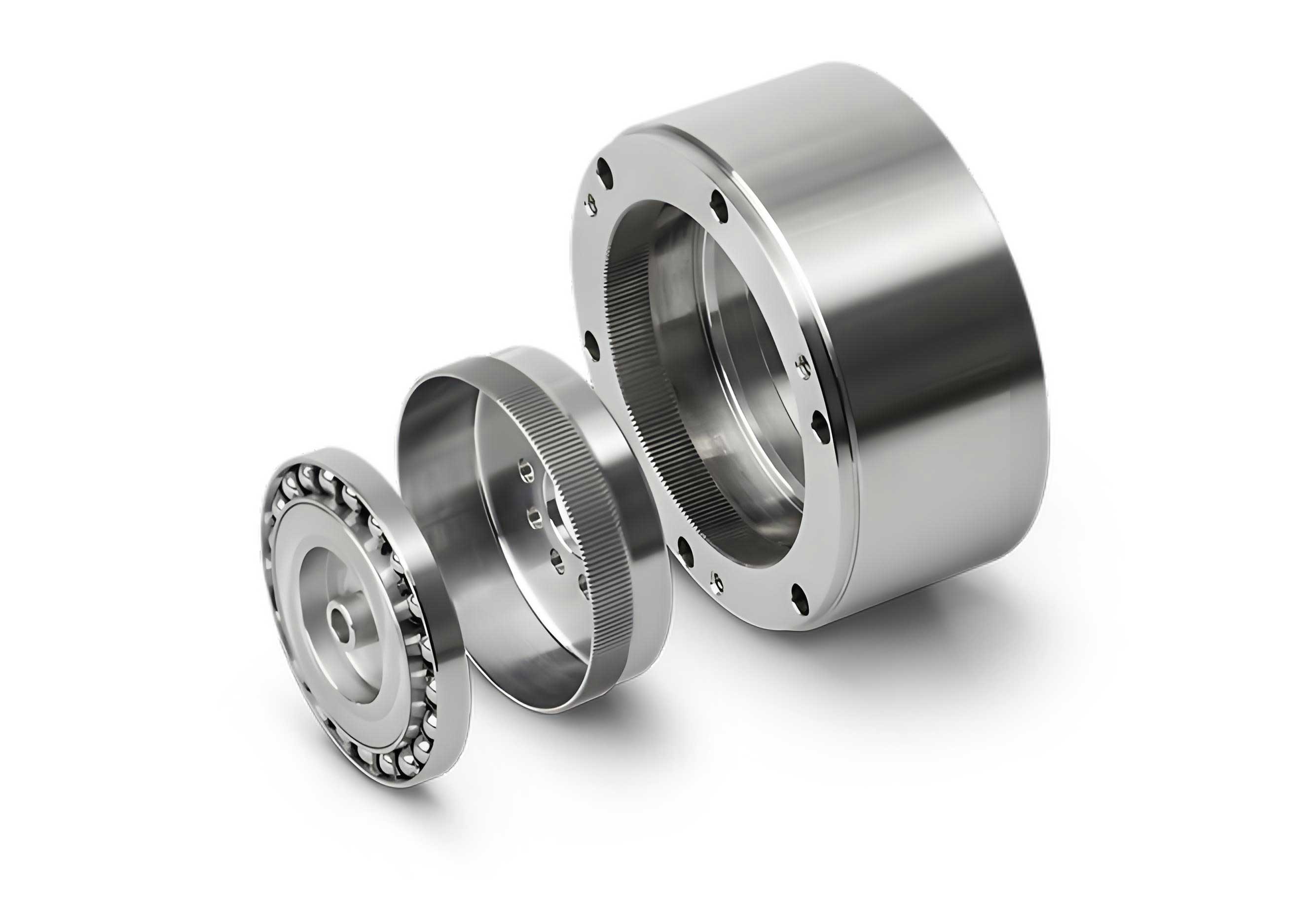
The unique operating principle of a harmonic drive gear involves the elastic deformation of the flexspline by an elliptical wave generator. This deformation creates two diametrically opposite regions of full engagement between the flexspline and circular spline teeth. As the wave generator rotates, these engagement zones travel around the circumference, producing a slow relative rotation between the two splines. The rate of this rotation is determined by the difference in the number of teeth between the flexspline (with more teeth) and the circular spline. The meshing behavior in these zones is not static but a dynamic process where conjugate action must be maintained despite the continuous deformation of the flexspline. This makes the choice of meshing parameters—primarily the profile shift coefficients of the flexspline and circular spline, and the radial deformation coefficient—critically important.
1. Mathematical Modeling for Backlash Calculation and Optimization
To formulate an optimization problem, we must first define a quantifiable measure of performance—the objective function—and identify the variables we can control. For a harmonic drive gear, the primary performance target related to meshing quality is the circumferential backlash, \( j_t \), measured at the reference circle.
1.1 Design Variables and Objective Function
The independent meshing parameters that significantly influence the backlash in a standardized harmonic drive gear are:
- The profile shift coefficient (or addendum modification coefficient) of the flexspline, \( x_1 \).
- The profile shift coefficient of the circular spline, \( x_2 \).
- The radial deformation coefficient, \( w_0^* = w_0 / m \), where \( w_0 \) is the radial deflection of the flexspline neutral line (wave generator amplitude) and \( m \) is the module.
Additionally, the meshing position, characterized by the polar angle \( U_H \) of a point on the cam (wave generator) profile, acts as an implicit parameter during the backlash calculation across the tooth profile. Therefore, we define a four-dimensional design variable vector:
$$ \mathbf{X} = [x_1, x_2, w_0^*, U_H]^T $$
The circumferential backlash \( j_t(\mathbf{X}) \) is not a single value but varies along the tooth depth in the engagement zone. It is defined as the minimum distance between non-working flanks of conjugate tooth profiles at a given mesh position. Therefore, we calculate it at several points \( k \) (where \( k = 1, 2, …, n_{uk} \)) along the flexspline tooth height and take the minimum:
$$ j_t(\mathbf{X}) = \min[ j_{tk}(\mathbf{X}) ], \quad (k=1,2,…,n_{uk}) $$
The number of calculation points \( n_{uk} \) is chosen to adequately sample the profile.
The core of the optimization is to find the vector \( \mathbf{X} \) that brings the calculated backlash \( j_t(\mathbf{X}) \) as close as possible to a desired target value \( j_c \), which is specified based on the harmonic drive gear’s application (e.g., \( j_c = 0 \) for precision positioning, \( j_c > 0 \) for power transmission). Consequently, the objective function \( F(\mathbf{X}) \) is formulated as the absolute deviation from this target:
$$ F(\mathbf{X}) = | j_t(\mathbf{X}) – j_c | $$
Thus, the optimization problem is formally stated as:
$$ \text{Find } \mathbf{X}^* \text{ that minimizes } F(\mathbf{X}) = | j_t(\mathbf{X}) – j_c | $$
subject to a set of geometric and performance constraints \( g_i(\mathbf{X}) \geq 0 \).
1.2 Backlash Calculation Formulation
Calculating \( j_{tk}(\mathbf{X}) \) requires determining the coordinates of corresponding points on the flexspline and circular spline tooth profiles in a fixed coordinate system. Consider a point \( K_1(X_{K1}, Y_{K1}) \) on the flexspline tooth profile. The conjugate point \( K_2(X_{K2}, Y_{K2}) \) on the neighboring circular spline tooth profile is found as the intersection of a circular arc centered at the origin with radius \( r_K = \sqrt{X_{K1}^2 + Y_{K1}^2} \). The circumferential backlash for this point-pair is the chordal distance:
$$ j_{tk} = \sqrt{ (X_{K1} – X_{K2})^2 + (Y_{K1} – Y_{K2})^2 } \tag{1} $$
The coordinates \( (X_{K1}, Y_{K1}) \) are derived by considering the flexspline’s deformation and rigid body motion. They are functions of the design variables and the profile parameter \( u_{K1} \):
$$
\begin{aligned}
X_{K1} &= r_1\{ \sin[\Psi – (u_{K1} – \xi_1)] + u_{K1}\cos\alpha\cos[\Psi – (u_{K1} – \xi_1 + \alpha)] \} + Q_1\sin\vartheta_1 – r_m\sin\Psi \\
Y_{K1} &= r_1\{ \cos[\Psi – (u_{K1} – \xi_1)] – u_{K1}\cos\alpha\sin[\Psi – (u_{K1} – \xi_1 + \alpha)] \} + Q_1\cos\vartheta_1 – r_m\cos\Psi
\end{aligned} \tag{2}
$$
Similarly, the coordinates of the circular spline point \( K_2 \) are:
$$
\begin{aligned}
X_{K2} &= r_2\{ \sin[\vartheta_2 – (u_{K2} – \xi_2)] + u_{K2}\cos\alpha\cos[\vartheta_2 – (u_{K2} – \xi_2 + \alpha)] \} \\
Y_{K2} &= r_2\{ \cos[\vartheta_2 – (u_{K2} – \xi_2)] – u_{K2}\cos\alpha\sin[\vartheta_2 – (u_{K2} – \xi_2 + \alpha)] \}
\end{aligned} \tag{3}
$$
Where:
- \( r_1, r_2 \): Pitch radii of flexspline and circular spline (\( r_i = 0.5 m z_i \)).
- \( \alpha \): Standard pressure angle at the pitch circle.
- \( \Psi \): Angular position of the flexspline neutral line point, related to \( U_H \) via the elliptical cam geometry: \( \Psi = \arctan\left(\frac{a^2}{b^2} \tan U_H\right) \), with \( a, b \) as the semi-major and semi-minor axes of the cam.
- \( \xi_1, \xi_2 \): Reference circle tooth thickness half-angles: \( \xi_1 = (\pi/2 + 2x_1\tan\alpha)/z_1 \), \( \xi_2 = (\pi/2 + 2x_2\tan\alpha)/z_2 \).
- \( Q_1, \vartheta_1 \): Radial distance and angle from cam center to flexspline neutral point.
- \( r_m \): Radius of the undeformed flexspline neutral line.
- \( \vartheta_2 \): Angular position of the circular spline: \( \vartheta_2 = \vartheta_1 z_1 / z_2 \).
- \( u_{K1}, u_{K2} \): Parameters of the involute curves for the flexspline and circular spline at points \( K_1 \) and \( K_2 \), calculated from the roll angles.
The profile parameters are calculated as follows, where \( r_{b1}, r_{b2} \) are the base circle radii:
$$ u_{K1} = \tan\left( \arccos\left( \frac{r_{b1}}{r_{u_{K1}}} \right) \right) – \tan\alpha = \text{inv}(\alpha_{K1}) \tag{4} $$
$$ u_{K2} = \tan\left( \arccos\left( \frac{r_{b2}}{r_K} \right) \right) – \tan\alpha = \text{inv}(\alpha_{K2}) \tag{5} $$
The radius \( r_{u_{K1}} \) for point \( K_1 \) is selected at uniform intervals along the flexspline tooth active height: \( r_{u_{K1}} = r_{a1} – (k-1) \cdot h_{uk} \), where \( h_{uk} = (r_{e1} – r_{s1})/(n_{uk}-1) \). The effective root radius of the flexspline \( r_{e1} \) and the tip radius of the circular spline \( r_{s1} \) are:
$$ r_{e1} = r_{a1} + w_0 = m(0.5z_1 + h_a^* + x_1) + m w_0^* \tag{6} $$
$$ r_{s1} = r_{a2} = m(0.5z_2 – h_a^* – c^* + x_2) \quad \text{(For clearance } c^*) \tag{7} $$
2. System Constraints for a Feasible Harmonic Drive Gear
The optimization search must be confined to a feasible region defined by constraints that ensure proper gear function, manufacturability, and avoidance of failure modes. The following constraints \( g_i(\mathbf{X}) \geq 0 \) are essential for any harmonic drive gear design.
| Constraint | Mathematical Expression \( g_i(\mathbf{X}) \geq 0 \) | Purpose |
|---|---|---|
| 1. Tooth Tip Thickness |
\( g_1(\mathbf{X}) = d_{a1} \left[ \frac{\pi + 4x_1\tan\alpha}{2z_1} + \text{inv}\alpha – \text{inv}\alpha_{a1} \right] – 0.25m \geq 0 \) \( d_{a2} \left[ \frac{\pi + 4x_2\tan\alpha}{2z_2} + \text{inv}\alpha – \text{inv}\alpha_{a2} \right] – 0.25m \geq 0 \) |
Prevents weakening of the tooth tip due to excessive pointing from large positive profile shift. |
| 2. Tip Interference Avoidance | \( g_2(\mathbf{X}) = \frac{X_{a2ea}}{Y_{a2ea}} – \frac{X_{a1ea}}{Y_{a1ea}} \geq 0 \) | Ensures the tips of the flexspline and circular spline do not collide during the meshing-in or meshing-out process. |
| 3. Minimum Engagement Depth | \( g_3(\mathbf{X}) = m[0.5(z_1 – z_2) + 2h_a^* + x_1 – x_2 + w_0^*] – m \geq 0 \) | Guarantees sufficient overlap of tooth profiles for effective load sharing and torque transmission. |
| 4. No Profile Overlap Interference | \( g_4(\mathbf{X}): X_{K2} – X_{K1} \geq 0 \quad \text{and} \quad Y_{K1} – Y_{K2} \geq 0 \) | Prevents the non-working flanks of adjacent teeth from intersecting at any point in the mesh cycle. |
| 5. Tip-Root Clearance | \( g_5(\mathbf{X}) = 0.5m(z_2 + h_a^* + c^* – x_2) – 0.5m(z_1 + h_a^* + x_1) – m w_0^* – 0.2m \geq 0 \) | Provides a safe radial clearance between the tip of one gear and the root of its mate at the deepest mesh point to account for deflections and thermal expansion. |
| 6. Flexspline Disengagement | \( g_6(\mathbf{X}) = m(z_1 + 2h_a^* + 2x_1) – m(z_2 + h_a^* – x_2) – 2.16 m w_0^* \geq 0 \) | Ensures the flexspline teeth can fully disengage from the circular spline teeth in the minor axis region of the wave generator. |
| 7. Undercut/Transition Curve Interference | \( g_7(\mathbf{X}): \quad r_{g2} – r_{a1} – m w_0^* \geq 0 \) \( \quad \quad \quad \quad r_{a2} – r_{g1} – m w_0^* \geq 0 \) |
Prevents the tip of one gear from contacting the non-involute fillet (transition curve) of the mating gear. |
| 8. Radial Deformation Range | \( g_8(\mathbf{X}): \quad w_0^* – 0.8 \geq 0 \quad \text{and} \quad 1.2 – w_0^* \geq 0 \) | Confines the radial deformation coefficient to a practical range for typical harmonic drive gear designs, balancing stress and engagement. |
The terms \( \alpha_{a1}, \alpha_{a2} \) are the pressure angles at the tip circles:
$$ \alpha_{a1} = \arccos\left( \frac{z_1 \cos\alpha}{z_1 + 2h_a^* + 2x_1} \right), \quad \alpha_{a2} = \arccos\left( \frac{z_2 \cos\alpha}{z_2 + 2h_a^* – 2x_2} \right) $$
The tip form radius \( r_g \) depends on the tool geometry and cutting conditions. For a gear generated by a rack-type cutter (typical for the flexspline), it is approximately:
$$ r_{g1} \approx m \sqrt{ (0.5z_1 – h_a^* + x_1)^2 + \left( \frac{(h_a^* – x_1)}{\tan\alpha} \right)^2 } \tag{8} $$
For the circular spline (internal gear) cut by a pinion-type cutter, the calculation is more complex and involves the cutting center distance \( a_{ce} \) and operating pressure angle \( \alpha_{ce} \):
$$ r_{g2} \approx \sqrt{ (a_{ce} \sin\alpha_{ce} + \sqrt{r_{a0}^2 – r_{b0}^2} )^2 + r_{b2}^2 } \tag{9} $$
where \( r_{a0}, r_{b0} \) are the tip and base radii of the cutter.
3. The Complex Method for Constrained Optimization
The formulated optimization problem is characterized by a non-analytic, computationally expensive objective function \( F(\mathbf{X}) \) and multiple nonlinear constraints \( g_i(\mathbf{X}) \). Gradient-based methods are unsuitable due to the difficulty in obtaining derivatives. The Complex Method, a direct search technique, is an excellent choice for solving this class of engineering design problems for a harmonic drive gear.
The algorithm operates within the feasible domain defined by the constraints. It starts by randomly generating an initial “complex” of \( k \) vertices (\( k > n+1 \), where \( n=4 \) is the number of design variables) within the feasible region. Each vertex represents a candidate set of meshing parameters \( \mathbf{X}_j \). The core iterative procedure is as follows:
- Evaluation: Compute the objective function \( F(\mathbf{X}_j) \) for each vertex in the complex.
- Identification: Find the worst vertex \( \mathbf{X}_w \) with the highest function value and the best vertex \( \mathbf{X}_b \) with the lowest.
- Centroid Calculation: Compute the centroid \( \mathbf{X}_c \) of all vertices except the worst:
$$ \mathbf{X}_c = \frac{1}{k-1} \sum_{j=1, j \neq w}^{k} \mathbf{X}_j $$ - Reflection: Generate a new trial point \( \mathbf{X}_r \) by reflecting the worst point through the centroid:
$$ \mathbf{X}_r = \mathbf{X}_c + \beta (\mathbf{X}_c – \mathbf{X}_w) $$
where \( \beta > 0 \) is the reflection coefficient (typically \( \beta = 1.3 \)). - Feasibility Check: If \( \mathbf{X}_r \) violates any constraint, move it halfway towards the centroid (\( \mathbf{X}_r = 0.5(\mathbf{X}_c + \mathbf{X}_r) \)) repeatedly until it becomes feasible.
- Replacement: If \( F(\mathbf{X}_r) < F(\mathbf{X}_w) \), replace \( \mathbf{X}_w \) with \( \mathbf{X}_r \). Otherwise, contract the reflection by moving \( \mathbf{X}_r \) halfway towards \( \mathbf{X}_c \) and check again. If it’s still not better, replace \( \mathbf{X}_w \) with \( \mathbf{X}_b \) plus a small random perturbation to restart the search locally.
- Convergence Check: Terminate the process when the standard deviation of the function values at all vertices, or the difference between best and worst, falls below a specified tolerance \( \epsilon \):
$$ \sqrt{ \frac{1}{k} \sum_{j=1}^{k} (F(\mathbf{X}_j) – \bar{F})^2 } < \epsilon $$
This method is robust because it uses only function evaluations, handles constraints directly by enforcing feasibility, and avoids premature convergence by maintaining a population of points. For the harmonic drive gear problem, the algorithm navigates the 4D parameter space (\( x_1, x_2, w_0^*, U_H \)) to find the combination that minimizes the backlash error \( |j_t – j_c| \).
4. Computational Implementation and Design Example
The optimization model and the Complex Method algorithm were implemented in computational software (e.g., MATLAB, Python). The process involves nested loops: an outer optimization loop managing the complex, and an inner analysis loop that, for a given \( \mathbf{X} \), calculates the backlash \( j_t(\mathbf{X}) \) by iterating over the tooth profile points \( k \) and the cam angle \( U_H \) to find the minimum gap.
To demonstrate the efficacy of this approach for a harmonic drive gear, consider a design case with the following fixed specifications:
| Parameter | Symbol | Value |
|---|---|---|
| Module | \( m \) | 0.25 mm |
| Pressure Angle | \( \alpha \) | 20° |
| Flexspline Tooth Count | \( z_1 \) | 200 |
| Circular Spline Tooth Count | \( z_2 \) | 202 |
| Addendum Coefficient | \( h_a^* \) | 1.0 |
| Number of Waves | \( n \) | 2 |
| Target Backlash | \( j_c \) | Nominally small (for high precision) |
The optimization was run with the constraints listed in Table 1. The Complex Method was initialized with \( k=10 \) vertices and a convergence tolerance \( \epsilon = 10^{-4} \).
| Optimized Meshing Parameter | Symbol | Optimal Value |
|---|---|---|
| Flexspline Profile Shift Coefficient | \( x_1 \) | 2.2950 |
| Circular Spline Profile Shift Coefficient | \( x_2 \) | 2.3184 |
| Radial Deformation Coefficient | \( w_0^* \) | 0.9980 |
| Implied Wave Generator Amplitude | \( w_0 = m w_0^* \) | 0.2495 mm |
A harmonic drive gear prototype was manufactured using these optimized parameters. Its critical performance metrics were tested and compared against the application requirements, which were stringent: transmission error < 3 arc-min, backlash < 3 arc-min, efficiency > 70%, and starting torque ≤ 6 N·cm.
| Performance Metric | Tested Value (Prototype) | Design Requirement | Status |
|---|---|---|---|
| Transmission Error | 2.75 arc-min | < 3 arc-min | Met |
| Backlash (Hysteresis) | 1.0 arc-min | < 3 arc-min | Met |
| Efficiency | 73% | > 70% | Met |
| Starting Torque | 2.62 N·cm | ≤ 6 N·cm | Met |
The results are conclusive. The harmonic drive gear manufactured with the optimized meshing parameters not only met but exceeded all key performance requirements. The very low achieved backlash of 1 arc-min, a direct outcome of the optimization targeting minimal functional clearance, validates the mathematical model and the optimization approach. The low transmission error and starting torque further confirm that the optimized parameters provide smooth, conjugate meshing action without undesirable interference or binding, which are common pitfalls in suboptimal harmonic drive gear designs.
5. Discussion and Conclusion
The design of a high-performance harmonic drive gear is a multidisciplinary challenge involving elasticity, contact mechanics, and gear geometry. This work has demonstrated that the critical first step—the selection of meshing parameters—can be effectively formulated and solved as a constrained nonlinear optimization problem. By explicitly defining the circumferential backlash as the objective function and incorporating comprehensive geometric constraints, the method ensures that the resulting harmonic drive gear design is not only optimal for the desired play but also feasible and robust against common failure modes.
The choice of the Complex Method proved highly suitable. Its ability to handle non-differentiable, simulation-based objective functions and explicit constraints makes it a practical tool for this real-world engineering problem. The significant positive profile shift coefficients (\( x_1, x_2 > 2.0 \)) obtained in the example are characteristic of harmonic drive gears. They serve to avoid undercut in the flexspline (which has a low virtual tooth count due to its large negative deflection), strengthen the tooth form, and, as optimized here, finely tune the operating clearance.
The radial deformation coefficient \( w_0^* \approx 1.0 \) is also typical, indicating a wave generator amplitude roughly equal to the module. This value balances sufficient tooth engagement for torque capacity against excessive flexspline stress and strain.
In conclusion, the systematic, optimization-based approach presented herein moves harmonic drive gear design from a realm of empirical trial-and-error or limited standard tables to a more analytical and performance-driven process. It allows designers to tailor a harmonic drive gear for specific applications, whether they demand ultra-high precision with near-zero backlash or robust power transmission with controlled clearance. Future work could expand the optimization framework to include multi-objective considerations, such as simultaneously minimizing backlash and maximizing fatigue life or torsional stiffness, further advancing the design sophistication of this uniquely capable gear technology.