
In the engineering of high-reliability systems, particularly within the demanding context of aerospace applications, the traditional paradigm of treating design parameters as deterministic values is fundamentally inadequate. The performance and longevity of critical components are invariably influenced by a multitude of uncertainties. These uncertainties, if not properly quantified and managed, can lead to significant errors in reliability predictions, potentially resulting in over-designed, wasteful systems or, more critically, under-designed systems prone to premature failure. This is especially true for precision components like the harmonic drive gear, which is ubiquitously employed in spacecraft mechanisms such as solar array drives and antenna pointing systems due to its exceptional qualities: high torque capacity, compactness and low mass, near-zero backlash, and a high single-stage reduction ratio. The reliable operation of these mechanisms over extended missions, often exceeding 15 years, is paramount, placing stringent requirements on the harmonic drive gear‘s durability. This article, from my perspective as a reliability analyst, delves into a sophisticated framework for assessing the reliability of a harmonic drive gear when confronted with the simultaneous presence of two distinct types of uncertainty: aleatory (inherent randomness) and epistemic (subjective lack of knowledge).
The core challenge in advanced reliability engineering lies in the appropriate characterization of uncertainty. Aleatory uncertainty, also known as objective or irreducible uncertainty, stems from the inherent randomness in physical processes or manufacturing variations. For instance, the precise yield strength of a batch of柔轮 (flexspline) material or the exact load experienced during a maneuver exhibits natural variability. This type of uncertainty is traditionally and effectively modeled using probability theory, where parameters are described by probability density functions (PDFs) derived from sufficient empirical data. In contrast, epistemic uncertainty arises from a deficiency of knowledge or information. This could be due to limited testing data for a new material, vague expert opinion on operational conditions, or unmodeled physical phenomena. For a harmonic drive gear operating in space, epistemic uncertainties abound: the exact degradation rate of lubrication under long-term vacuum and radiation, the precise value of an application-specific service factor, or the bounds of an unexpected resonant frequency. When data is sparse, purely probabilistic models can be misleading, as they may impose a specific distribution shape (e.g., normal) on parameters without justifiable evidence. Therefore, a hybrid approach that marries probabilistic methods for aleatory variables with non-probabilistic methods for epistemic variables offers a more robust and honest representation of the state of knowledge.
This study focuses on developing and demonstrating a probability-nonprobability mixed reliability model. The epistemic uncertainties, due to lack of data, will be represented using interval analysis, where a parameter is known only to lie within a bounded range, e.g., $Y^I = [\underline{Y}, \overline{Y}]$. The aleatory uncertainties, with sufficient statistical backing, will be modeled as random variables following defined distributions, e.g., $X \sim N(\mu_X, \sigma_X^2)$. The performance function, or limit state function $G(\mathbf{X}, \mathbf{Y})$, which defines failure ($G<0$) and safe ($G>0$) regions, will thus be a function of both random vector $\mathbf{X}$ and interval vector $\mathbf{Y}$. The goal is to compute the bounds of the system’s failure probability $P_f$, which will itself be an interval $[P_f^{min}, P_f^{max}]$, reflecting the influence of the epistemic uncertainty. A significant advantage of the proposed method is its avoidance of the iterative “Most Probable Point (MPP)” search required by classical First-Order Reliability Methods (FORM), which can be computationally intensive and non-robust for highly nonlinear or implicit limit states. Instead, a sampling-and-regression approach focused on the vicinity of the limit state is employed to approximate the failure boundary, enhancing robustness and computational efficiency.
1. Representation and Propagation of Uncertain Information
1.1 Probabilistic Modeling of Aleatory Uncertainty
When ample data exists, parameters can be treated as random variables. The probability of failure is defined as the integral of the joint PDF over the failure domain:
$$ P_f = P[G(\mathbf{X}) < 0] = \int_{G(\mathbf{x})<0} f_{\mathbf{X}}(\mathbf{x}) d\mathbf{x} $$
For correlated non-normal variables, transformations like the Nataf transformation are used to map them into a standard uncorrelated normal space $\mathbf{U}$ for analysis. The First-Order Reliability Method (FORM) linearizes the limit state in this U-space at the MPP. However, the need for gradient calculations and iterative MPP search can be a drawback. As an alternative, one can use a direct sampling-based approach. By generating a strategic set of samples $\{\mathbf{x}^{(k)}\}$ that satisfy $G(\mathbf{x}^{(k)}) \approx 0$, a linear approximation (a hyperplane) $G_L(\mathbf{X}) = 0$ of the true limit state can be constructed via regression. The failure probability assessed using this hyperplane often provides an excellent and computationally efficient approximation, as the samples capturing the most likely failure region are used to define it.
In practice, even for “aleatory” parameters, the true distribution parameters (e.g., the mean $\mu$) might be uncertain if data is limited. Bayesian estimation is a powerful tool to refine such estimates by combining prior knowledge with new data. If a parameter $\theta$ has a prior distribution $\pi(\theta)$ and new data $\mathbf{x}$ is observed with likelihood $p(\mathbf{x}|\theta)$, the posterior distribution, representing our updated belief, is proportional to their product:
$$ \pi(\theta | \mathbf{x}) \propto p(\mathbf{x}|\theta) \pi(\theta) $$
For example, the mean value of a service factor $K_A$ can be updated this way, moving from a prior estimate (perhaps from a handbook) to a posterior estimate informed by specific test data or expert judgment for the spacecraft application.
1.2 Interval-Based Modeling of Epistemic Uncertainty
For parameters where only a range of possible values can be ascertained, interval mathematics provides a straightforward and rigorous framework. An interval variable $Y^I$ is defined as:
$$ Y^I = [\underline{Y}, \overline{Y}] = \{ y \in \mathbb{R} \ | \ \underline{Y} \le y \le \overline{Y} \} $$
where $\underline{Y}$ and $\overline{Y}$ are the lower and upper bounds, respectively. When multiple, possibly conflicting, sources of information are available (e.g., two different expert opinions, two testing methods), they must be aggregated into a single interval representation. Common aggregation operations include:
| Operation | Definition | Description |
|---|---|---|
| Union | $Y^I = [\min(y_1^-,…,y_n^-), \max(y_1^+,…,y_n^+)]$ | Captures the entire range from all sources. The most conservative approach. |
| Average | $Y^I = \left[ \frac{1}{n}\sum_{i=1}^n y_i^-,\ \frac{1}{n}\sum_{i=1}^n y_i^+ \right]$ | Finds the mean interval, balancing different sources. |
| Weighted Mixture | $Y^I = \left[ \sum_{i=1}^n w_i y_i^-,\ \sum_{i=1}^n w_i y_i^+ \right],\ \sum w_i=1$ | Combines intervals with different confidence weights $w_i$. |
For a system described solely by interval parameters $\mathbf{Y}$, a non-probabilistic reliability index $\eta$ can be defined. If the system performance function is $Z = G(\mathbf{Y})$, and its interval midpoint (center) and radius are $Z_c$ and $Z_r$ respectively, the reliability index is:
$$ \eta = \frac{Z_c}{Z_r} $$
The criterion is: if $\eta > 1$, the system is reliably safe; if $\eta < -1$, it is reliably failed; and if $-1 \le \eta \le 1$, the safety state is indeterminate due to the epistemic uncertainty—the system could be either safe or failed.
2. The Probability-Nonprobability Hybrid Reliability Model
The real analytical challenge emerges when both types of uncertainty coexist within a single system model. Consider a general limit state function $G(\mathbf{X}, \mathbf{Y})$, where $\mathbf{X}$ is a vector of $m$ random variables (aleatory) and $\mathbf{Y}$ is a vector of $n$ interval variables (epistemic). The failure probability $P_f$ is no longer a single value but becomes dependent on the specific realization of $\mathbf{Y}$ within its interval. Therefore, we seek the bounds of $P_f$ as $\mathbf{Y}$ varies over its domain: $P_f^{min}$ and $P_f^{max}$.
To illustrate the formulation, consider a linear limit state function, which could be the linear approximation $G_L(\cdot)$ obtained from regressing samples near a more complex function:
$$ G_L(\mathbf{X}, \mathbf{Y}) = \sum_{i=1}^{m} a_i X_i + \sum_{j=1}^{n} b_j Y_j + a_0 $$
where $X_i \sim N(\mu_{X_i}, \sigma_{X_i}^2)$ and $Y_j \in [\underline{Y_j}, \overline{Y_j}]$. The center and radius of the interval $Y_j$ are $Y_{j,c} = (\underline{Y_j}+\overline{Y_j})/2$ and $Y_{j,r} = (\overline{Y_j}-\underline{Y_j})/2$.
For a given fixed vector $\mathbf{y}$ (a realization of $\mathbf{Y}$), the function becomes $G_L(\mathbf{X}, \mathbf{y}) = \sum a_i X_i + \text{constant}$, and its reliability index $\beta$ is:
$$ \beta(\mathbf{y}) = \frac{\sum_{i=1}^{m} a_i \mu_{X_i} + \sum_{j=1}^{n} b_j y_j + a_0}{\sqrt{\sum_{i=1}^{m} (a_i \sigma_{X_i})^2}} $$
Since $y_j$ can vary within $[Y_{j,c} – Y_{j,r},\ Y_{j,c} + Y_{j,r}]$, the reliability index $\beta$ becomes an interval. The minimum and maximum values of $\beta$ are found by minimizing/maximizing the numerator:
$$ \beta_{min} = \frac{\sum a_i \mu_{X_i} + \sum b_j Y_{j,c} – \sum |b_j| Y_{j,r} + a_0}{\sqrt{\sum (a_i \sigma_{X_i})^2}} $$
$$ \beta_{max} = \frac{\sum a_i \mu_{X_i} + \sum b_j Y_{j,c} + \sum |b_j| Y_{j,r} + a_0}{\sqrt{\sum (a_i \sigma_{X_i})^2}} $$
The corresponding bounds on failure probability for the linearized limit state are:
$$ P_f^{max} \approx \Phi(-\beta_{min}), \quad P_f^{min} \approx \Phi(-\beta_{max}) $$
where $\Phi(\cdot)$ is the standard normal cumulative distribution function. The true failure probability of the original system lies within this interval: $P_f \in [P_f^{min},\ P_f^{max}]$. The region between the hyperplanes defined by $\beta_{min}$ and $\beta_{max}$ represents the uncertain domain influenced by epistemic variables.
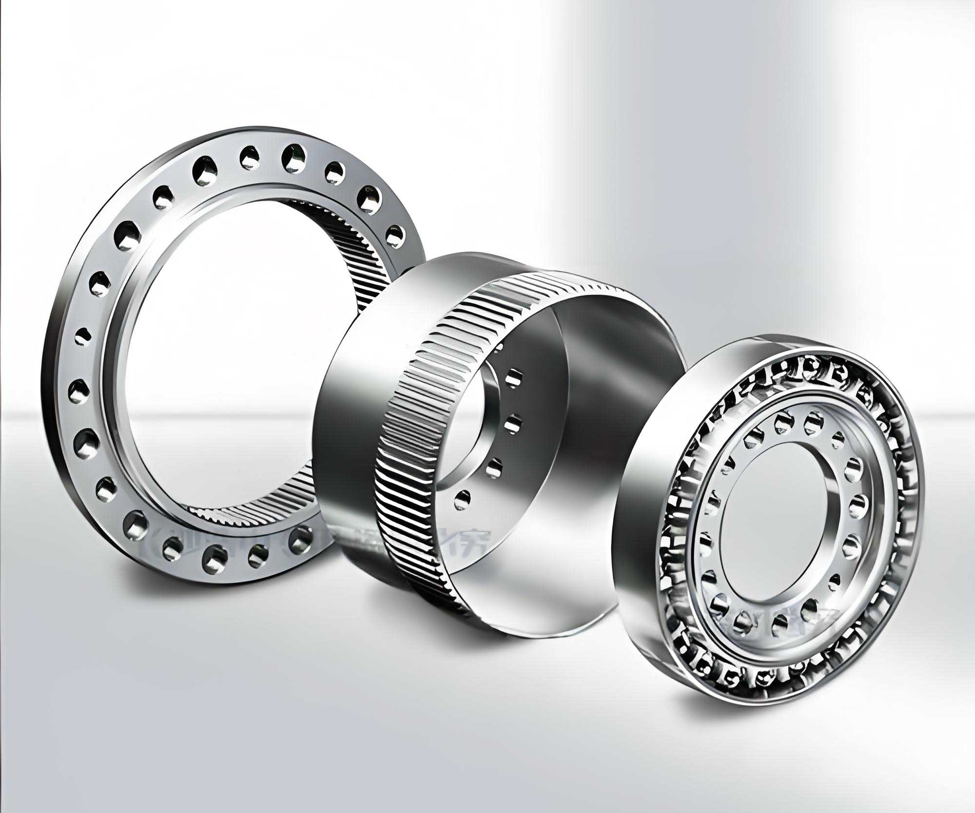
3. Reliability Modeling of a Spacecraft Harmonic Drive Gear
The harmonic drive gear is a critical component, and its life often dictates the service life of the entire mechanism. A common empirical model for the expected life $L_h$ (in hours) of a harmonic drive gear is:
$$ L_h = \left( \frac{3.575 \times 10^7}{N_V \cdot K_A \cdot T} \cdot T_H \right)^3 $$
where:
$T_H$ = Rated output torque (N·m)
$N_V$ = Actual input speed (rpm)
$T$ = Output shaft nominal torque (N·m)
$K_A$ = Application service factor (dimensionless)
$m$ = Design life in years
Converting this to a limit state function for reliability analysis over a mission life of $m$ years (where 1 year = 8760 hours), we define:
$$ G(T_H, N_V, T, K_A, m) = L_h – 8760 \cdot m = \left( \frac{3.575 \times 10^7 \cdot T_H}{N_V \cdot K_A \cdot T} \right)^3 – 8760 \cdot m $$
Failure occurs when $G < 0$ (calculated life less than required life), and safety when $G > 0$.
In a traditional deterministic analysis, one might plug in fixed nominal values. For example, with $T_H=350$ N·m, $N_V=0.1$ rpm, $T=2000$ N·m, $K_A=1.3$, and $m=15$ years, we get $G \approx 13100 > 0$, suggesting a reliable design. This is misleading, as it ignores uncertainty.
A more rigorous analysis classifies the variables based on available information. For a spacecraft harmonic drive gear:
– Aleatory Variables (Random): $T_H$ and $K_A$. Sufficient historical manufacturing and test data might allow us to model $T_H$ as Normal: $T_H \sim N(\mu_{T_H}, \sigma_{T_H}^2)$. The service factor $K_A$ is also subject to variability and can be modeled as $K_A \sim N(\mu_{K_A}, \sigma_{K_A}^2)$. If $\mu_{K_A}$ is uncertain, Bayesian updating can be used to refine its estimate from a prior distribution and new application-specific data.
– Epistemic Variables (Interval): $N_V$ and $T$. The operational speed $N_V$ may vary within a range due to changing mission profiles and environmental factors, but its exact probability distribution is unknown—only bounds can be estimated: $N_V \in [\underline{N_V}, \overline{N_V}]$. Similarly, the output torque $T$ is highly dependent on dynamic spacecraft maneuvers and disturbances, best described by an interval: $T \in [\underline{T}, \overline{T}]$.
Thus, the limit state becomes $G(\mathbf{X}, \mathbf{Y})$, with $\mathbf{X} = [T_H, K_A]^T$ and $\mathbf{Y} = [N_V, T]^T$. The failure probability will be an interval.
4. Case Study: Numerical Implementation and Sensitivity Analysis
Let’s implement the hybrid model with the following assumed data, representative of a spacecraft harmonic drive gear application.
| Variable | Distribution Type | Mean ($\mu$) | Std. Dev. ($\sigma$) | Notes |
|---|---|---|---|---|
| $T_H$ (Rated Torque) | Normal | 350 N·m | 35 N·m | From manufacturer test data. |
| $K_A$ (Service Factor) | Normal | $\mu_{K_A}$ (Bayesian Estimate) | 0.1 | Mean is updated from prior. |
Assume a prior for $\mu_{K_A}$ is $N(1.268, 0.08^2)$. Incorporating a new expert judgment suggesting $K_A=1.35$ as a likely value, the Bayesian posterior mean is calculated as $\hat{\mu}_{K_A} \approx 1.3$.
| Variable | Source 1 | Source 2 | Aggregated Interval (Average) | Aggregated Interval (Union) |
|---|---|---|---|---|
| $T$ (Output Torque) | [1900, 2150] N·m | [1900, 2080] N·m | [1900, 2115] N·m | [1900, 2150] N·m |
| $N_V$ (Input Speed) | [0.095, 0.112] rpm | [0.085, 0.108] rpm | [0.090, 0.110] rpm | [0.085, 0.112] rpm |
For this analysis, we will use the “Average” aggregated intervals: $T^I = [1900, 2115]$ N·m and $N_V^I = [0.090, 0.110]$ rpm. Their midpoints and radii are: $T_c=2007.5, T_r=107.5$; $N_{V,c}=0.10, N_{V,r}=0.01$.
The first step is to approximate the nonlinear limit state function $G(\cdot)$ with a linear function $G_L(\cdot)$ near the failure boundary. Using a focused sampling strategy around $G \approx 0$ and linear regression, we obtain an approximation. For instance, around a 15-year life, the linearized function might take the form:
$$ G_L \approx a_0 + a_1 T_H + a_2 K_A + a_3 T + a_4 N_V $$
Suppose regression yields: $a_0 = -1.02\times10^6$, $a_1 = 3200$, $a_2 = -8.5\times10^5$, $a_3 = -540$, $a_4 = -1.08\times10^7$. (Note: Coefficients are illustrative; actual values depend on the sampling region).
We can now compute the reliability index bounds. The denominator for $\beta$ is:
$$ \sigma_{G_L} = \sqrt{(a_1 \sigma_{T_H})^2 + (a_2 \sigma_{K_A})^2} = \sqrt{(3200 \times 35)^2 + (-8.5\times10^5 \times 0.1)^2} $$
The numerator varies with the interval parameters. Using the formulas for $\beta_{min}$ and $\beta_{max}$:
$$ \beta_{max} = \frac{a_1\mu_{T_H} + a_2\mu_{K_A} + a_0 + a_3 T_c + a_4 N_{V,c} + |a_3|T_r + |a_4|N_{V,r}}{\sigma_{G_L}} $$
$$ \beta_{min} = \frac{a_1\mu_{T_H} + a_2\mu_{K_A} + a_0 + a_3 T_c + a_4 N_{V,c} – |a_3|T_r – |a_4|N_{V,r}}{\sigma_{G_L}} $$
The corresponding failure probability bounds are $P_f^{max} = \Phi(-\beta_{min})$ and $P_f^{min} = \Phi(-\beta_{max})$. Calculating these for different design lives $m$ (which affects the intercept $a_0$ via the regression) yields the following results:
| Design Life, $m$ (years) | $\beta_{min}$ | $\beta_{max}$ | $P_f^{min}$ | $P_f^{max}$ |
|---|---|---|---|---|
| 10 | 1.23 | 2.39 | 0.009 | 0.109 |
| 11 | 0.99 | 2.16 | 0.015 | 0.161 |
| 12 | 0.76 | 1.94 | 0.026 | 0.224 |
| 13 | 0.55 | 1.73 | 0.042 | 0.291 |
| 14 | 0.34 | 1.53 | 0.063 | 0.366 |
| 15 | 0.15 | 1.34 | 0.090 | 0.440 |
The results are striking. While a naive deterministic calculation showed no issue at 15 years, the hybrid uncertainty analysis reveals a failure probability between 9% and 44%. This wide interval, particularly the high upper bound, underscores the critical impact of epistemic uncertainty (the unknown precise values of $T$ and $N_V$) on the reliability assessment. A decision-maker must consider this range, perhaps targeting a design modification or seeking more information to reduce the interval width.
To validate the accuracy of the linear approximation method, a large-scale Monte Carlo Simulation (MCS) with $10^6$ samples was performed for the 15-year case, directly evaluating the original nonlinear limit state function. The MCS results yielded $P_f^{min}_{MCS} \approx 0.088$ and $P_f^{max}_{MCS} \approx 0.446$, showing excellent agreement with the proposed method’s results of 0.090 and 0.440. The proposed method achieves this with significantly lower computational cost, as it avoids evaluating millions of samples for the full nonlinear function and instead relies on a small, strategic set for regression.
4.1 Sensitivity Analysis
Understanding which parameters most influence the failure probability is crucial for guiding design improvements and data collection efforts. Sensitivity analysis for the hybrid model examines the rate of change of the failure probability bounds with respect to distribution parameters (for random variables) and interval bounds.
For the random variables ($T_H$, $K_A$), we compute the sensitivity of the average failure probability $\bar{P}_f = (P_f^{min}+P_f^{max})/2$. The derivatives with respect to the mean $\mu_i$ and standard deviation $\sigma_i$ of variable $X_i$ are approximated using the concepts from FORM, adapted for the two bounding hyperplanes:
$$ \frac{\partial \bar{P}_f}{\partial \mu_i} \approx -\frac{1}{2} \left[ \frac{\varphi(-\beta_{min})}{\sigma_{G_L}} \cdot a_i \cdot \alpha_{i,min} + \frac{\varphi(-\beta_{max})}{\sigma_{G_L}} \cdot a_i \cdot \alpha_{i,max} \right] $$
$$ \frac{\partial \bar{P}_f}{\partial \sigma_i} \approx -\frac{1}{2} \left[ \frac{\varphi(-\beta_{min})}{\sigma_{G_L}} \cdot (a_i \sigma_i) \cdot (\alpha_{i,min}^2 – 1) + \frac{\varphi(-\beta_{max})}{\sigma_{G_L}} \cdot (a_i \sigma_i) \cdot (\alpha_{i,max}^2 – 1) \right] $$
where $\varphi$ is the standard normal PDF, and $\alpha_{i,min}, \alpha_{i,max}$ are the direction cosines for the two hyperplanes. For interval variables, a finite difference approach is used, perturbing their bounds:
$$ \frac{\partial \bar{P}_f}{\partial B} \approx \frac{\bar{P}_f(B + \Delta B) – \bar{P}_f(B)}{\Delta B} $$
where $B$ represents $\underline{Y_j}$ or $\overline{Y_j}$.
The sensitivity results for the 15-year design life case are summarized below:
| Parameter | Sensitivity $\partial \bar{P}_f / \partial (\cdot)$ | Interpretation |
|---|---|---|
| Mean of $T_H$, $\mu_{T_H}$ | -6.2 × 10⁻⁷ per N·m | Increasing the mean rated torque decreases failure probability (negative sensitivity). The effect is very small. |
| Std. Dev. of $T_H$, $\sigma_{T_H}$ | 2.8 × 10⁻⁸ per (N·m) | Increasing variability in $T_H$ slightly increases $P_f$. |
| Mean of $K_A$, $\mu_{K_A}$ | 0.047 per unit | A very strong positive sensitivity. Increasing the mean service factor (making the design condition more severe) drastically increases failure probability. |
| Std. Dev. of $K_A$, $\sigma_{K_A}$ | 0.447 per unit | The strongest sensitivity. Reducing uncertainty ($\sigma_{K_A}$) in the service factor is the most effective way to reduce $P_f$ and its uncertainty band. |
| Output Torque $T$ (Upper Bound $\overline{T}$) | 0.0016 per N·m | Increasing the maximum expected output torque increases $P_f$. |
| Input Speed $N_V$ (Upper Bound $\overline{N_V}$) | 15.2 per rpm | Extremely high sensitivity. The operational speed $N_V$ is the most critical epistemic parameter. Precise knowledge and control of its maximum value are paramount. |
The sensitivity analysis delivers clear guidance: the reliability of the spacecraft harmonic drive gear is most sensitive to the application service factor $K_A$ (particularly its uncertainty) and the upper bound of the operational input speed $N_V$. Design efforts should therefore prioritize: 1) Obtaining more precise, application-tuned data to reduce the uncertainty in $K_A$, potentially moving it from an uncertain random variable to a better-characterized one. 2) Implementing tighter control or more accurate prediction of the operational speed range $N_V$ to reduce its epistemic interval width. Reducing these uncertainties will shrink the $[P_f^{min}, P_f^{max}]$ interval and provide a much clearer picture of the harmonic drive gear‘s true reliability.
5. Conclusion
The analysis of a harmonic drive gear for long-life spacecraft applications necessitates a reliability framework that can explicitly handle both aleatory and epistemic uncertainties. Treating all parameters as fixed values or even as purely random variables can lead to significant underestimation of risk when knowledge is incomplete. The probability-nonprobability hybrid model presented here, utilizing interval analysis for epistemic uncertainty, provides a rigorous and practical solution. It quantifies the effect of incomplete knowledge by producing bounded failure probability estimates, offering decision-makers a more complete risk profile. The application to the harmonic drive gear life model convincingly demonstrated that deterministic analysis can be dangerously optimistic, while the hybrid model reveals a potentially wide range of failure probabilities dependent on poorly known operational parameters. The accompanying sensitivity analysis pinpoints the parameters whose uncertainty most heavily influences the system reliability, directing valuable engineering resources towards obtaining better information or implementing design controls. Furthermore, the methodological approach of approximating the limit state via regression on strategically sampled points proves to be computationally efficient and robust, circumventing the convergence issues sometimes associated with MPP search algorithms. This framework is not limited to harmonic drive gear analysis but is broadly applicable to the reliability assessment of any complex system where data scarcity and inherent variability coexist, especially in the demanding field of aerospace engineering.