
The strain wave gear, a pivotal innovation in precision transmission, operates on the principle of controlled elastic deformation. At its heart lies the flexible spline (flexspline), a thin-walled cup that is deformed by a wave generator into a non-circular shape to engage with a rigid circular spline (circular spline). The accurate representation of the deformed neutral line (or middle surface) of the flexspline’s tooth rim is the foundational step for conjugate tooth profile design, directly influencing the transmission’s precision, load capacity, and backlash characteristics. Traditional methods, relying on the superposition of radial, circumferential, and rotational displacements derived from small-deformation ring theory, introduce positioning errors for gear teeth due to inherent assumptions and the neglect of nonlinear effects. This article presents a first-person perspective on a geometric feature interpolation method, developed to express the deformed neutral line more accurately by directly considering its final shape, boundary conditions, and circumferential elongation.
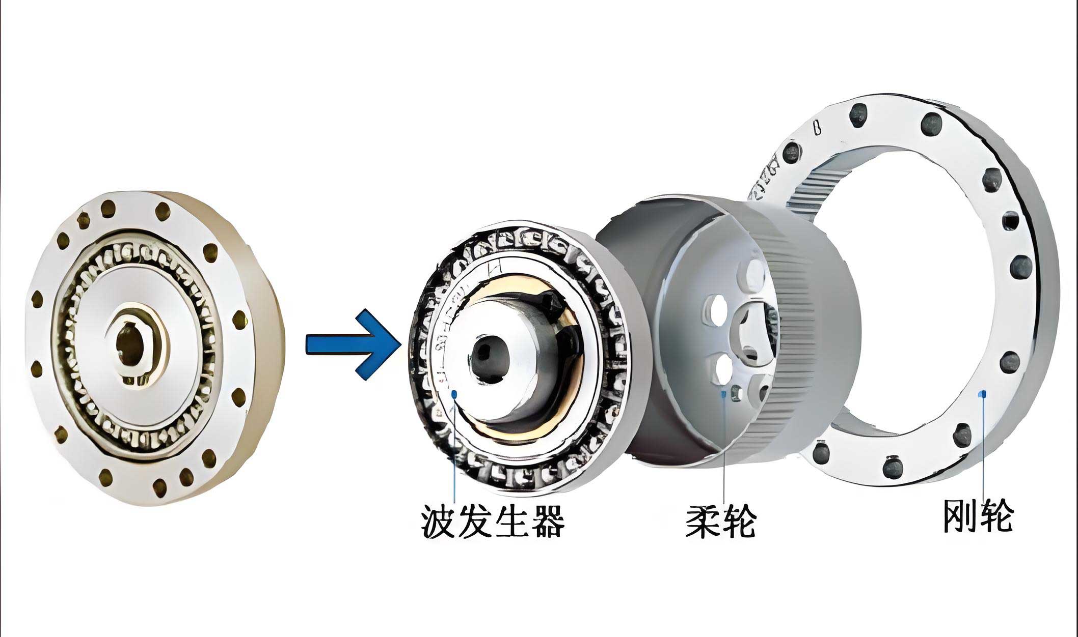
The core of the strain wave gear assembly is the interaction between the wave generator and the flexspline. For a common double-disk cam type wave generator, the theoretical cam profile is composed of two circular arcs. The initial, undeformed neutral line of the flexspline’s tooth rim is a perfect circle. Upon assembly, the cam forces the flexspline to conform to its shape over a certain contact region, known as the wrap angle (\(\gamma\)). Outside this wrap angle, the flexspline deforms freely under the action of bending moments and circumferential forces. The objective is to derive a continuous mathematical expression for the entire deformed neutral line from the long axis to the short axis.
The Deformation Model and Its Parameters
Establishing the geometric and kinematic relationships is the first step. Let \( O_1 \) be the center of the deformed flexspline (coinciding with the wave generator’s rotation center), \( r_m \) the initial radius of the neutral line circle, and \( u_0 \) the maximum radial displacement at the long axis. The theoretical cam profile radius is \( R = R_1 + s_c + s_1/2 \), where \( R_1 \) is the disk radius, \( s_c \) the bushing thickness, and \( s_1 \) the flexspline wall thickness. The eccentricity \( e \) is given by:
$$ e = r_m + u_0 – R $$
The wrap angle \( \gamma \) on the deformed neutral line corresponds to a different central angle \( \gamma_0 \) on the initial undeformed circle due to circumferential strain. Their relationship, considering the geometry of the contact arc, is:
$$ \gamma_0 = \gamma_1 \frac{R}{r_m} $$
where \( \gamma_1 \) is the central angle subtended by the contact arc \( CB’ \) on the cam profile:
$$ \gamma_1 = \gamma + \arcsin\left(\frac{e \sin \gamma}{R}\right) $$
Consequently, the arc length of the contact region is:
$$ \widehat{CB’} = \gamma_1 R $$
The coordinates of the boundary point \( B’ \) between the contact and free regions, in the global coordinate system \( O_1-xy \), are:
$$ x_{B’} = R \sin \gamma_1, \quad y_{B’} = e + R \cos \gamma_1 $$
Geometric Feature Interpolation Method for the Neutral Line
The proposed method abandons the displacement superposition approach. Instead, it treats the deformed neutral line in two distinct segments, applying strict geometric continuity and physical constraints to derive its final form.
1. Deformation Function in the Contact Region
Within the wrap angle (\(0 \le \phi \le \gamma\), where \(\phi\) is measured from the long axis), the neutral line is assumed to be in perfect, strain-free contact with the cam profile. Therefore, its shape is simply the offset curve (isometric line) of the cam at a distance equal to half the wall thickness. For the theoretical calculation, it is the cam profile itself. In the \(O_1-xy\) system, this is given by the circle:
$$ x^2 + (y – e)^2 = R^2, \quad x \in [0, x_{B’}] $$
Here, the wrap angle \(\gamma\) is an unknown to be solved simultaneously with the free segment’s equations.
2. Deformation Function in the Non-Contact Region
For the free deformation region (\( \gamma \le \phi \le \pi/2 \)), we establish a local polar coordinate system \( O-x_1y_1 \) with its origin at \( O_1 \) and the \( y_1 \)-axis passing through point \( B’ \). Let \( \theta \) be the polar angle in this system, ranging from \( 0 \) at \( B’ \) to \( \eta = \pi/2 – \gamma \) at the short axis point \( A’ \).
We propose to express the neutral line in this region as a polynomial in \( \theta \):
$$ \rho(\theta) = \sum_{i=0}^{n} C_i \theta^i, \quad \theta \in [0, \eta] $$
where \( \rho \) is the radial distance. To uniquely determine the coefficients \( C_i \) and the unknown wrap angle \( \gamma \), we need a number of constraint equations equal to the number of unknowns. With \( \gamma \) unknown, we set \( n=4 \), requiring five coefficients (\( C_0 \) to \( C_4 \)) and thus six constraints (one of which will solve for \( \gamma \)).
The six constraints are derived from geometry and mechanics:
Constraint 1: Continuity at Point \( B’ \). The coordinates of \( B’ \) must satisfy both the contact circle and the polynomial.
$$ \rho(0) = C_0 = \sqrt{x_{B’}^2 + y_{B’}^2} = \frac{R \sin \gamma_1}{\sin \gamma} $$
Constraint 2: Slope Continuity (Smoothness) at Point \( B’ \). The neutral line must be smooth at the transition. The slope of the contact circle at \( B’ \) is \( k_1 = -\tan(\gamma_1 – \gamma) \). The slope from the polynomial is \( k_2 = (dy_1/dx_1) \). Equating them at \( \theta=0 \) yields:
$$ \left. \frac{dy_1}{dx_1} \right|_{\theta=0} = \frac{\rho'(0)}{\rho(0)} = -\tan(\gamma_1 – \gamma) \implies C_1 = -C_0 \tan(\gamma_1 – \gamma) $$
where \( \rho'(0) = C_1 \).
Constraint 3: Curvature Continuity at Point \( B’ \). The curvature radius must also be continuous. The curvature radius of the contact circle is \( R \). The general formula for curvature radius in polar coordinates is:
$$ R_{curve}(\theta) = \frac{ \left( \rho^2 + \rho’^2 \right)^{3/2} }{ \rho^2 + 2\rho’^2 – \rho \rho” } $$
Setting \( R_{curve}(0) = R \), and knowing \( \rho”(0) = 2C_2 \), we get:
$$ \frac{ (C_0^2 + C_1^2)^{3/2} }{ C_0^2 + 2C_1^2 – 2 C_0 C_2 } = R \implies C_2 = \frac{ R(C_0^2 + 2C_1^2) – (C_0^2 + C_1^2)^{3/2} }{ 2 R C_0 } $$
Constraint 4: Slope Condition at Point \( A’ \) (Short Axis). At the short axis (\(\phi = \pi/2\) or \(\theta = \eta\)), the tangent to the neutral line is vertical. In the \( O-x_1y_1 \) system, this slope is \( k_{A’} = -1/\tan \gamma \). Applying this condition gives a relation between coefficients:
$$ \left. \frac{dy_1}{dx_1} \right|_{\theta=\eta} = \frac{ \rho'(\eta) + \rho(\eta)\tan \gamma }{ \rho'(\eta)\tan \gamma – \rho(\eta) } = -\frac{1}{\tan \gamma} $$
This can be solved to express \( C_3 \) in terms of the other coefficients and \( \eta \):
$$ C_3 = -\frac{ C_1 + 2C_2\eta + 4C_4\eta^3 }{ 3\eta^2 } $$
Constraint 5: Curvature Condition at Point \( A’ \). Obtaining the exact deformed curvature at the short axis is complex. As a practical and reasonable approximation, we use the curvature derived from the small-deformation theory’s displacement superposition method. First, solve for the theoretical small-deformation wrap angle \( \gamma_s \) from:
$$ \frac{u_0 B_1}{A_1 – B_1} = r_m^2 \left( \frac{1}{R} – \frac{1}{r_m} \right) $$
where \( A_1 = \eta_1 – \sin\gamma_s \cos\gamma_s \), \( B_1 = \frac{4}{\pi}(\cos\gamma_s – \eta_1 \sin\gamma_s) \), and \( \eta_1 = \pi/2 – \gamma_s \).
Then, the radial displacement \( u(\phi) \) from the small-deformation theory gives the polar radius \( \rho_1(\phi) = r_m + u(\phi) \). Its first and second derivatives, \( \rho_1′(\phi) \) and \( \rho_1”(\phi) \), are calculated. The curvature radius at the short axis (\( \phi = \pi/2 \)) is:
$$ R_{A’} = \frac{ \rho_1^2(\pi/2) }{ \rho_1(\pi/2) – \rho_1”(\pi/2) } $$
We then enforce that the curvature radius from our polynomial at \( \theta=\eta \) equals \( R_{A’} \):
$$ \frac{ \left[ \rho^2(\eta) + \rho’^2(\eta) \right]^{3/2} }{ \rho^2(\eta) + 2\rho’^2(\eta) – \rho(\eta)\rho”(\eta) } = R_{A’} $$
Substituting the expressions for \( C_0, C_1, C_2, C_3 \) (all functions of \( \gamma \)) and \( C_4 \) into this equation yields a nonlinear equation: \( C_4 = g(\gamma) \).
Constraint 6: Arc Length Condition (Circumferential Elongation). The total length of the deformed neutral line in one quadrant must equal the initial length plus the elongation caused by the circumferential tensile force. The arc length of the free region from the polynomial is:
$$ \widehat{B’A’} = \int_{0}^{\eta} \sqrt{ \rho^2 + \rho’^2 } \, d\theta $$
The total deformed arc length is \( \widehat{CB’} + \widehat{B’A’} = \gamma_1 R + \int_{0}^{\eta} \sqrt{ \rho^2 + \rho’^2 } \, d\theta \).
The initial arc length is \( r_m \pi/2 \). The elongation \( \Delta S \) for one quadrant, derived from mechanical analysis considering circumferential force, is:
$$ \Delta S = \frac{s_1^2 u_0}{6 r_m^2} \cdot \frac{ 1 – r_m(1 – r_m/R)/u_0 }{ \eta – \sin\gamma \cos\gamma } (\gamma \sin\gamma + \cos\gamma) $$
Thus, the arc length constraint is:
$$ \gamma_1 R + \int_{0}^{\eta} \sqrt{ \rho^2(\theta) + \rho’^2(\theta) } \, d\theta = r_m \frac{\pi}{2} + \Delta S $$
This is another nonlinear equation in \( \gamma \) and \( C_4 \).
Constraints 5 and 6 form a system of two nonlinear equations with unknowns \( \gamma \) and \( C_4 \). They are solved iteratively, using the small-deformation theory wrap angle \( \gamma_s \) as an initial guess for \( \gamma \).
Model Solving and Numerical Verification
To validate the geometric interpolation method, a series of models with varying wrap angles were constructed by changing the cam radius \( R \) while keeping \( r_m = 61.7 \, \text{mm} \) and \( u_0 = 0.7 \, \text{mm} \) constant. Finite Element Analysis (FEA) models of the ring in contact with the cam were developed in a plane-stress environment. Crucially, analyses were performed under both small deformation and large deformation (geometric nonlinearity) assumptions. The large deformation FEA results, which account for the significant shape change and nonlinear contact, are considered the most accurate reference for real-world behavior.
The following table summarizes the calculated polynomial coefficients and the solved wrap angle \( \gamma \) for various models using the geometric interpolation method.
| Model | \(C_0\) | \(C_1\) | \(C_2\) | \(C_3\) | \(C_4\) | Wrap Angle \(\gamma\) (°) |
|---|---|---|---|---|---|---|
| 1 | 62.3852 | -0.3267 | -1.7979 | 1.2381 | -0.1919 | 5.1899 |
| 2 | 62.3746 | -0.4191 | -1.7209 | 1.2381 | -0.1967 | 6.9375 |
| 3 | 62.3615 | -0.5055 | -1.6496 | 1.2417 | -0.2024 | 8.7010 |
| … | … | … | … | … | … | … |
| 9 | 62.0507 | -1.2583 | -1.0367 | 1.5694 | -0.3667 | 30.9529 |
| 10 | 61.8480 | -1.4765 | -0.8372 | 1.9608 | -0.5611 | 40.8325 |
| 11 | 61.6054 | -1.6525 | -0.6455 | 2.7599 | -1.0297 | 51.0796 |
| 12 | 61.3323 | -1.7817 | -0.4594 | 4.6502 | -2.4758 | 61.4399 |
| 13 | 61.2001 | -1.8233 | -0.3753 | 6.3983 | -4.1059 | 66.1987 |
Comparison of Wrap Angle Results
The solved wrap angles from four different methods—Displacement Superposition Theory, FEA Small Deformation, FEA Large Deformation, and the Geometric Interpolation Method—were compared. The deviation of each method’s result from the FEA Large Deformation benchmark is plotted against the wrap angle from the geometric method.
The key finding is that both the Displacement Superposition Theory and FEA Small Deformation results show significant and growing deviations from the large deformation benchmark as the model wrap angle increases. In contrast, the results from the Geometric Interpolation Method align almost perfectly with the FEA Large Deformation results for a wide range of wrap angles, specifically between approximately 25° and 65°. For very small wrap angles (below ~25°), the small-deformation-based methods show stable, smaller errors, while the geometric method has larger initial deviations.
Comparison of Short Axis Length
The radial coordinate of the short axis point \( A’ \) (the minor axis length) is another critical parameter. The following table and analysis show the deviation of this parameter calculated by different methods from the FEA Large Deformation result.
The trend is consistent: the geometric method provides results very close to the large deformation FEA for models with wrap angles between 25° and 65°. Outside this range, especially for larger wrap angles, its deviation increases, though it may still be better than the displacement superposition method.
Gear Tooth Positioning Accuracy
In strain wave gear design, gear teeth are positioned on the deformed neutral line. Errors in the neutral line description translate directly into tooth positioning errors. We analyze the polar angle and polar radius of equally spaced points on the initial circle after deformation. For a model with a 30° wrap angle (a common design range), the geometric method’s superiority is evident.
Polar Angle Deviation: The geometric method shows nearly zero deviation across the entire quadrant. The FEA Small Deformation method has a maximum deviation of about 0.004°, while the Displacement Superposition Theory shows a maximum deviation of approximately 0.0058°.
Polar Radius Deviation: In the contact region, both the geometric method and FEA Small Deformation show minimal error. In the free region, the geometric method’s deviation remains stable below 0.001 mm. The Displacement Superposition Theory, however, shows a deviation that grows towards the short axis, reaching a maximum. The geometric method reduces the maximum polar radius deviation by about 0.013 mm compared to the displacement superposition method in this 30° wrap angle model.
| Performance Metric | Displacement Superposition | FEA Small Deformation | Geometric Interpolation | FEA Large Deformation (Benchmark) |
|---|---|---|---|---|
| Max Polar Angle Error | ~0.0058° | ~0.004° | <0.0001° | 0° (Reference) |
| Max Polar Radius Error | ~0.013 mm (at short axis) | ~0.008 mm (at short axis) | <0.001 mm | 0 mm (Reference) |
| Applicability Range | Best for γ < 25° | Best for γ < 25° | Best for 25° ≤ γ ≤ 65° | Accurate for all γ (Computationally expensive) |
Discussion and Application
The geometric feature interpolation method effectively decouples the complex nonlinear contact and large deformation problem. By fixing the contact region to the cam profile and using geometric continuity and a physical elongation constraint to solve for the free region, it eliminates the cumulative errors inherent in the sequential displacement superposition process. This method is particularly advantageous for strain wave gear designs with moderate wrap angles, which often correspond to optimal assembly stress conditions.
The procedure for applying this method in strain wave gear design can be summarized as follows:
- Define Input Parameters: Initial neutral line radius \( r_m \), wall thickness \( s_1 \), max radial displacement \( u_0 \), and cam parameters (disk radius \( R_1 \), bushing thickness \( s_c \)).
- Iterative Solution: Solve the system of nonlinear equations (Constraints 5 & 6) for the true wrap angle \( \gamma \) and the polynomial coefficient \( C_4 \). Use the small-deformation theory angle \( \gamma_s \) as the initial guess.
- Construct Neutral Line: For \( 0 \le \phi \le \gamma \), use the circle equation \( \rho(\phi) = \sqrt{R^2 – e^2 \sin^2 \phi} – e \cos \phi \). For \( \gamma \le \phi \le \pi/2 \), calculate \( \theta = \phi – \gamma \) and use \( \rho(\theta) = C_0 + C_1\theta + C_2\theta^2 + C_3\theta^3 + C_4\theta^4 \).
- Tooth Positioning: Map the initial, equally spaced tooth center points from the undeformed circle to this deformed neutral line profile using the solved geometric description for highly accurate conjugate tooth profile generation.
The method’s main limitation is its reduced accuracy for very small wrap angles, where the small-deformation assumptions are more valid, and for very large wrap angles where the fourth-order polynomial may be insufficient to capture extreme curvature changes. Future work could explore higher-order polynomials or piecewise splines for the free region and integrate more sophisticated mechanical models for the short-axis curvature condition.
Conclusion
Accurate description of the flexspline’s deformed neutral line is paramount for high-performance strain wave gear design. The traditional displacement superposition method, while useful, introduces non-negligible errors due to its underlying small-deformation assumptions. The geometric feature interpolation method presented here provides a compelling alternative. By directly constructing the final shape based on geometric continuity, curvature conditions, and circumferential elongation, it yields a neutral line representation that closely matches the results of computationally intensive, nonlinear large deformation FEA for a practical range of wrap angles (25° to 65°). This method enhances the accuracy of gear tooth positioning, which is the cornerstone of precise conjugate tooth profile design, ultimately contributing to the development of strain wave gears with higher transmission accuracy, load capacity, and longevity. The strain wave gear, reliant on this precise elastic deformation, thus benefits significantly from a geometrically rigorous approach to defining its core deformation geometry.