
In the field of precision motion control and robotic systems, the strain wave gear, also known as harmonic drive, plays a pivotal role due to its compact design, high reduction ratios, and minimal backlash. As a key transmission component in industrial robots and aerospace equipment, the dynamic performance and accuracy of strain wave gears directly influence the overall system performance. However, the inherent nonlinearities, such as hysteretic stiffness and dynamic friction, pose significant challenges for accurate dynamic analysis and control. Traditional models often simplify these aspects by treating stiffness as constant or piecewise constant and friction as static, leading to reduced precision in dynamic predictions. In this study, we aim to address these limitations by developing a comprehensive nonlinear dynamic model for strain wave gears that incorporates memory-based hysteretic stiffness and LuGre dynamic friction. Through extensive simulation, we explore the effects of various parameters on system output, providing insights for design optimization and performance enhancement. This work contributes to the advancement of high-precision transmission systems by offering a more realistic representation of strain wave gear dynamics.
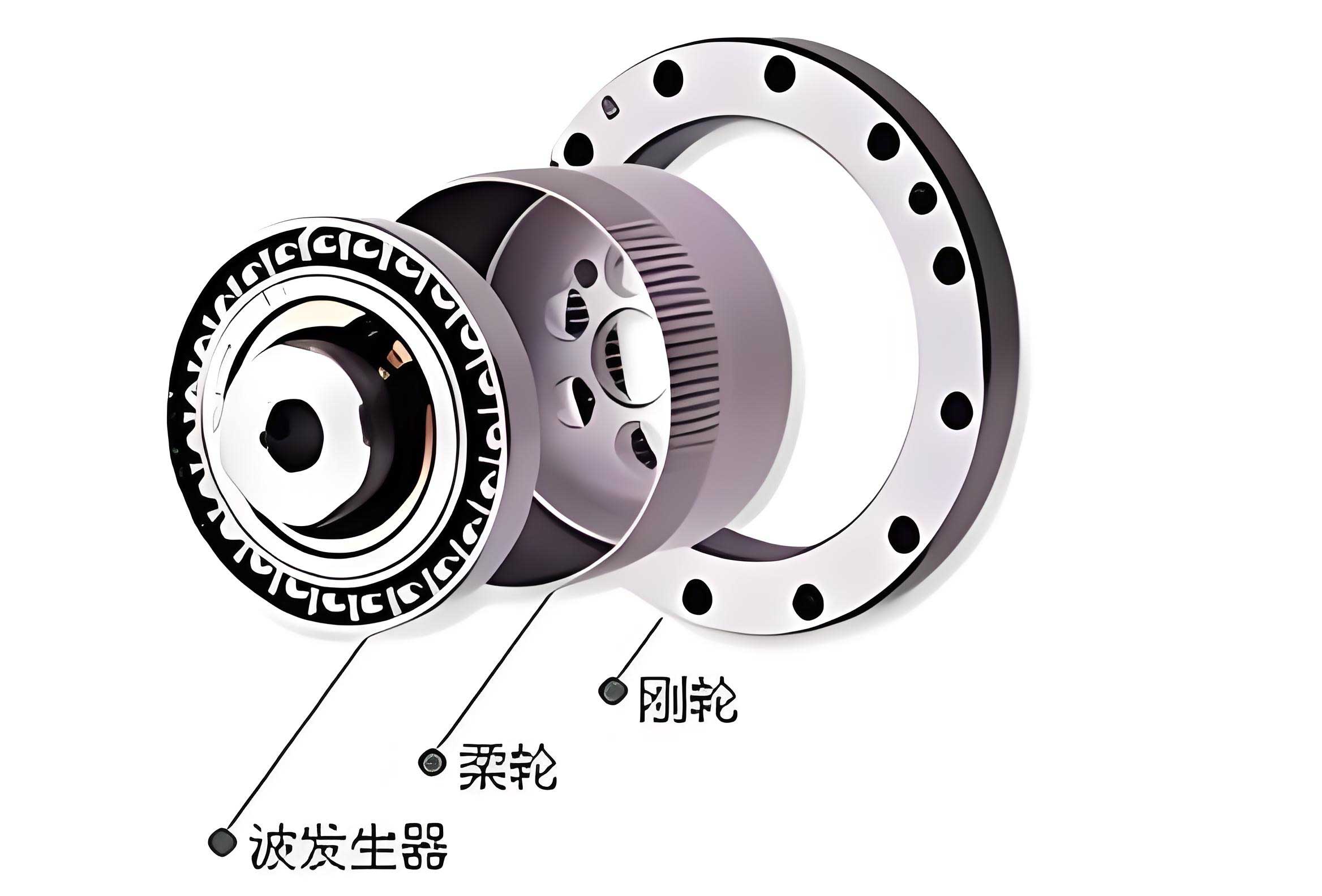
The strain wave gear operates on the principle of elastic deformation, where a flexible spline (flexspline) meshes with a rigid circular spline (circular spline) via a wave generator. This unique mechanism results in complex interactions that exhibit nonlinear behaviors, including stiffness hysteresis and friction dynamics. These nonlinearities are not merely perturbations but fundamental attributes that affect torque transmission, efficiency, and stability. Over the years, researchers have developed various models to capture the dynamics of strain wave gears, ranging from linear approximations to sophisticated nonlinear frameworks. Early models, such as the second-order linear model pioneered by Soviet scholars, provided a foundation but overlooked critical nonlinear effects. Subsequent studies introduced factors like transmission error, nonlinear damping, and hysteresis, yet often in a simplified manner. For instance, some models represented hysteresis using segmented stiffness or static friction models, which fail to account for the path-dependent nature and dynamic transitions observed in real systems. Our approach builds upon these works by integrating a memory-based hysteretic stiffness model and a LuGre dynamic friction model, both of which are grounded in physical phenomena and validated through simulation. By doing so, we strive to improve the accuracy of dynamic analysis for strain wave gears, ultimately aiding in the design of more reliable and efficient transmission systems.
The core of our modeling effort lies in the representation of hysteretic stiffness. Hysteresis, or memory effect, refers to the dependency of the system output not only on the current input but also on the history of inputs. In the context of strain wave gears, this manifests as a relationship between transmitted torque and torsional angle that forms closed loops during loading and unloading cycles. To model this, we adopt a memory-based approach where the stiffness is described as a nonlinear function with a correction term that accounts for past states. Let $\theta(t)$ denote the torsional angle at time $t$, defined as the difference between the motor-side angular displacement $\theta_j$ and the load-side angular displacement $\theta_z$, scaled by the gear ratio $N$:
$$ \theta(t) = \frac{\theta_j}{N} – \theta_z $$
The transmitted torque $T$ is expressed as a sum of a nonlinear function $f(\theta)$ and a memory term $z$:
$$ T(\theta, t) = f(\theta) + z = f(\theta) + \int_0^t \phi(x) \dot{\theta}(x) dx $$
Here, $\phi(x)$ is a memory factor that decays over time, capturing the fading influence of past states. We define it as an exponential function:
$$ \phi(x) = A e^{-Bx} $$
where $A$ and $B$ are parameters that characterize the memory strength and decay rate. The function $f(\theta)$ represents the static stiffness curve, which we model as a cubic polynomial to reflect the increasing stiffness with torque:
$$ f(\theta) = a\theta^3 + b\theta^2 + c\theta $$
Assuming a periodic torsional angle $\theta(t) = C \sin(\omega t)$, the memory term $z$ can be derived analytically, leading to the complete expression for transmitted torque:
$$ T(\theta, t) = a\theta^3 + b\theta^2 + c\theta \pm \left[ \frac{AC\omega – AC(B \sin \omega t + \omega \cos \omega t)e^{-Bt}}{B^2 + \omega^2} \right] $$
The sign depends on the direction of angular velocity. The nonlinear transmission stiffness $K(t)$ is then obtained as the derivative:
$$ K(t) = \frac{dT(t)}{d\theta(t)} = \frac{dT(t)}{dt} \left( \frac{1}{\dot{\theta}} \right) $$
This model effectively captures the hysteresis loops observed in strain wave gears, where stiffness varies with both torque magnitude and loading history.
Another critical nonlinearity in strain wave gears is dynamic friction, which arises primarily from the meshing between the flexspline and circular spline, as well as from bearings and other contacts. Static friction models, such as Coulomb or Stribeck models, are insufficient because they ignore dynamic effects like presliding displacement, frictional memory, and the Stribeck effect. To address this, we employ the LuGre (Lund-Grenoble) dynamic friction model, which conceptualizes friction as the average deflection of elastic bristles at the contact surface. The LuGre model is governed by the following equations:
$$ \frac{ds}{dt} = \omega – \frac{|\omega|}{g(\omega)} s $$
$$ g(\omega) = \frac{1}{\sigma_0} \left[ T_c + (T_s – T_c) e^{-(\omega/\omega_s)^2} \right] $$
$$ T_f = \sigma_0 s + \sigma_1 \frac{ds}{dt} $$
Here, $s$ is the average bristle deflection, $\omega$ is the relative angular velocity between the mating surfaces (approximated as the flexspline angular velocity when the circular spline is fixed), $g(\omega)$ is the Stribeck function, $\omega_s$ is the Stribeck velocity, $\sigma_0$ is the bristle stiffness, $\sigma_1$ is the micro-damping coefficient, $T_c$ is the Coulomb friction torque, and $T_s$ is the static friction torque. The friction torque $T_f$ contributes to the damping in the system, and the nonlinear damping coefficient $C_0(t)$ is derived as:
$$ C_0(t) = \frac{dT_f(t)}{d\omega(t)} = \frac{dT_f(t)}{dt} \left( \frac{1}{\ddot{\theta}_z} \right) $$
The LuGre model seamlessly transitions between static and dynamic friction regimes, incorporating phenomena like stick-slip and velocity-dependent friction, making it suitable for high-precision applications involving strain wave gears.
Integrating the hysteretic stiffness and dynamic friction models, we formulate the overall dynamic model of a strain wave gear transmission system. The system comprises a servo motor, a strain wave gear reducer, an inertial load, and associated sensors. The wave generator is driven by the motor, and the flexspline outputs motion to the load. The torque balance equations are derived based on the schematic representation of torque transmission, where the strain wave gear is simplified as a parallel combination of a nonlinear spring (representing stiffness) and a damper (representing friction). The equations of motion are as follows:
$$ J_j \ddot{\theta}_j + C_j \dot{\theta}_j = T_j – T_a $$
$$ J_z \ddot{\theta}_z + C_z \dot{\theta}_z = T_b $$
$$ T_b = K \left( \frac{\theta_j}{N} – \theta_z \right) $$
$$ N T_a = T_b + T_f = T_b + C_0 \dot{\theta}_j $$
where $J_j$ and $J_z$ are the motor-side and load-side moments of inertia, $C_j$ and $C_z$ are the motor-side and load-side damping coefficients, $K$ is the transmission stiffness coefficient (now a function of time in the full model), $C_0$ is the nonlinear damping coefficient from friction, $N$ is the gear ratio, $T_j$ is the motor torque, $T_a$ is the input torque to the wave generator, and $T_b$ is the output torque from the flexspline. For a DC servo motor, the motor dynamics are described by:
$$ T_j = K_m i – T_1 $$
$$ u = i R + K_e \dot{\theta}_j $$
with $K_m$ as the motor torque constant, $K_e$ as the back-EMF constant, $u$ as the input voltage, $i$ as the armature current, $R$ as the armature resistance, and $T_1$ as the no-load torque. Combining these, the system differential equations become:
$$ J_j \ddot{\theta}_j + C_j \dot{\theta}_j = \frac{K_m}{R} (u – K_e \dot{\theta}_j) – \frac{K}{N} \left( \frac{\theta_j}{N} – \theta_z \right) – \frac{C_0 \dot{\theta}_j}{N} $$
$$ J_z \ddot{\theta}_z + C_z \dot{\theta}_z = K \left( \frac{\theta_j}{N} – \theta_z \right) $$
To analyze system behavior, we derive the transfer function by neglecting damping and considering an equivalent constant stiffness $\bar{K}$, resulting in:
$$ G(s) = \frac{\theta_z(s)}{U(s)} = \frac{\bar{K} K_m N}{J_j J_z N^2 R s^4 + J_z K_a K_m N^2 s^3 + \bar{K} N R (J_j N + J_z) s^2 + \bar{K} K_a K_m N^2 s + \bar{K} R (\bar{K} N – \bar{K})} $$
where $K_a$ is a combined constant. This linearized model provides a baseline, but the full nonlinear model is essential for accurate dynamic analysis.
To validate our nonlinear dynamic model, we developed a simulation framework using Matlab Simulink. The simulation model implements the differential equations with integrated subsystems for hysteretic stiffness and dynamic friction. The block diagram of the strain wave gear system was constructed to represent the interactions between motor, gear, and load dynamics. Key parameters were selected based on typical strain wave gear specifications and motor characteristics, as summarized in Table 1. These values serve as the foundation for our simulation studies, allowing us to investigate the effects of nonlinearities and parameter variations.
| Parameter | Symbol | Value | Unit |
|---|---|---|---|
| Armature Resistance | $R$ | 6 | $\Omega$ |
| Motor Torque Constant | $K_m$ | 0.52 | N·m/A |
| Back-EMF Constant | $K_e$ | 0.52 | V·s/rad |
| Motor Damping Coefficient | $C_j$ | 0.003 | kg·m²·s⁻¹·rad⁻¹ |
| Load Damping Coefficient | $C_z$ | 0.005 | kg·m²·s⁻¹·rad⁻¹ |
| Gear Equivalent Damping Coefficient | $C$ | 0.16 | kg·m²·s⁻¹·rad⁻¹ |
| Gear Ratio | $N$ | 100 | – |
| Equivalent Stiffness | $\bar{K}$ | 7.8 × 10⁵ | N·m/rad |
| Motor-Side Inertia | $J_j$ | 6.8 × 10⁻⁴ | kg·m² |
| Load-Side Inertia | $J_z$ | 2.4 × 10⁻² | kg·m² |
The hysteretic stiffness subsystem was implemented using the memory-based model with parameters $A = 40000$, $B = 300$, $a = 0.12$, $b = 0.56$, and $c = 52000$. For the dynamic friction model, due to the complexity of parameter identification, we initially treated $C_0$ as a constant in some simulations to isolate effects, but the LuGre model structure was retained for future refinement. The input voltage was set to a 24 V, 50 Hz sinusoidal signal to excite the system dynamics, and simulations were run to observe the load-side angular displacement $\theta_z$ over time.
The simulation results revealed several important insights. Under the 24 V sinusoidal input, the load-side angular displacement reached a maximum at approximately $t = 0.054$ s and then stabilized around $\theta_z = 0.1096^\circ$ with minor oscillations. This behavior indicates the system’s dynamic response to periodic excitation. When incorporating the hysteretic stiffness model, the stiffness curve exhibited a closed hysteresis loop, converging to a symmetric cycle around the origin. The instantaneous stiffness $K(t)$ fluctuated near $7 \times 10^5$ N·m/rad, confirming the model’s ability to replicate hysteresis phenomena. Comparative analysis showed that the model with hysteretic stiffness produced slightly lower steady-state angular displacements than the equivalent constant stiffness model, demonstrating that stiffness hysteresis reduces system output and transmission efficiency. This efficiency loss is attributed to energy dissipation within the hysteresis loop, often referred to as hysteresis loss.
We further investigated the impact of input voltage variations. Increasing the input voltage amplitude while keeping frequency constant resulted in higher load-side angular displacements and larger oscillation ranges, although the oscillation period remained unchanged. This suggests that higher input energies amplify output motions but also exacerbate dynamic instabilities, highlighting the need for careful voltage regulation in strain wave gear applications. To quantify parameter influences, we conducted parametric studies by varying the transmission stiffness coefficient $K$ and damping torque coefficient $C_0$ independently. The trends are summarized below:
- Transmission Stiffness ($K$): Higher stiffness values led to increased system stability, with reduced oscillations and higher output displacements. Conversely, lower stiffness caused output decline and tendencies toward instability, as the system’s natural frequency shifted closer to excitation frequencies, potentially inducing resonance.
- Damping Torque Coefficient ($C_0$): Larger damping coefficients reduced load-side angular displacements, indicating lower transmission efficiency. This is because increased damping dissipates more energy as heat, diminishing the torque available for output motion.
These findings underscore the trade-offs in strain wave gear design: maximizing stiffness enhances stability and output, while minimizing damping improves efficiency. Practical measures to achieve this include using high-strength alloy steels for gear components, optimizing tooth profiles, and selecting advanced lubricants to reduce friction. Additionally, structural improvements, such as enhanced flexspline designs, can further mitigate hysteresis and friction effects.
The integration of nonlinear models for hysteretic stiffness and dynamic friction represents a significant advancement over traditional linear or piecewise models. Our memory-based hysteresis model captures the path-dependent nature of stiffness, while the LuGre friction model accounts for dynamic transitions between friction states. Together, they provide a more accurate depiction of strain wave gear dynamics, which is crucial for high-precision applications like robotic joints and aerospace actuators. Future work could focus on experimental validation of these models, parameter identification techniques for the LuGre model, and the development of model-based control strategies to compensate for nonlinearities. Moreover, extending the model to include other effects, such as thermal influences or wear over time, would enhance its applicability to real-world scenarios.
In conclusion, this study presents a comprehensive nonlinear dynamic model for strain wave gears, incorporating memory-based hysteretic stiffness and LuGre dynamic friction. Through simulation, we demonstrated that hysteresis reduces output and efficiency, while higher stiffness promotes stability and lower damping improves efficiency. These insights guide the design and optimization of strain wave gear systems for improved performance. As demand for precision motion control grows, accurate dynamic models like ours will play an increasingly vital role in advancing transmission technology. The strain wave gear, with its unique advantages, continues to be a focus of innovation, and our work contributes to a deeper understanding of its complex dynamics.
To further elaborate on the modeling aspects, we can express the hysteretic stiffness behavior using differential equations. The memory term $z$ satisfies a first-order differential equation derived from its integral form. Defining $z$ as:
$$ \dot{z} = A e^{-Bt} \dot{\theta} – B z $$
This formulation facilitates numerical implementation in simulation environments. Similarly, the LuGre model equations can be discretized for real-time applications. The complexity of these models necessitates computational tools, but they offer fidelity that simpler models lack. In terms of system performance metrics, we define transmission efficiency $\eta$ as the ratio of output power to input power, which can be expressed as:
$$ \eta = \frac{T_b \dot{\theta}_z}{T_j \dot{\theta}_j} $$
Under hysteresis, this efficiency decreases due to energy losses in the stiffness loop. Our simulations approximate this efficiency reduction, though exact quantification requires detailed loss analysis.
Another key consideration is the effect of gear ratio $N$ on dynamics. Higher ratios amplify torque but also introduce more nonlinearities due to increased flexspline deformation. Our model accounts for this through the torsional angle definition. Sensitivity analysis could explore optimal gear ratios for specific applications, balancing torque output with dynamic response.
In practice, strain wave gears are often used in closed-loop control systems. Our model can be linearized around operating points for controller design, but the full nonlinear model should be used for simulation-based verification. Techniques like feedback linearization or adaptive control may mitigate nonlinear effects, improving tracking accuracy. For instance, a controller that compensates for hysteresis and friction could use inverse models based on our formulations.
From a broader perspective, the advancements in strain wave gear modeling contribute to the field of mechatronics, where mechanical and electrical systems are tightly integrated. As robots become more dexterous and aerospace systems more autonomous, the need for precise transmission models will only increase. Our work aligns with this trend, offering a robust framework for dynamic analysis. We encourage researchers and engineers to adopt such nonlinear models to push the boundaries of what strain wave gears can achieve in high-performance applications.
Ultimately, the journey toward perfecting strain wave gear dynamics is ongoing. Each improvement in modeling brings us closer to systems that are efficient, stable, and precise. By embracing complexity rather than simplifying it, we pave the way for innovations that will define the future of motion transmission. The strain wave gear, a marvel of engineering, deserves nothing less than models that capture its true essence, and we believe our contribution is a step in that direction.