
The rotary vector reducer, a sophisticated two-stage planetary speed reducer, represents a pinnacle of precision power transmission technology. Characterized by its compact structure, high torque density, exceptional positional accuracy, and smooth operation, it has become the indispensable drive component in advanced industrial robots and precision machinery. Its architecture ingeniously combines a first-stage involute planetary gear train with a second-stage cycloidal pin gear drive. This analysis delves into the fundamental kinematic and static force principles governing the rotary vector reducer, followed by a systematic evaluation of the influence of key design parameters on its meshing force characteristics using an osculating value method.
1. Kinematic Analysis and Reduction Ratio Derivation
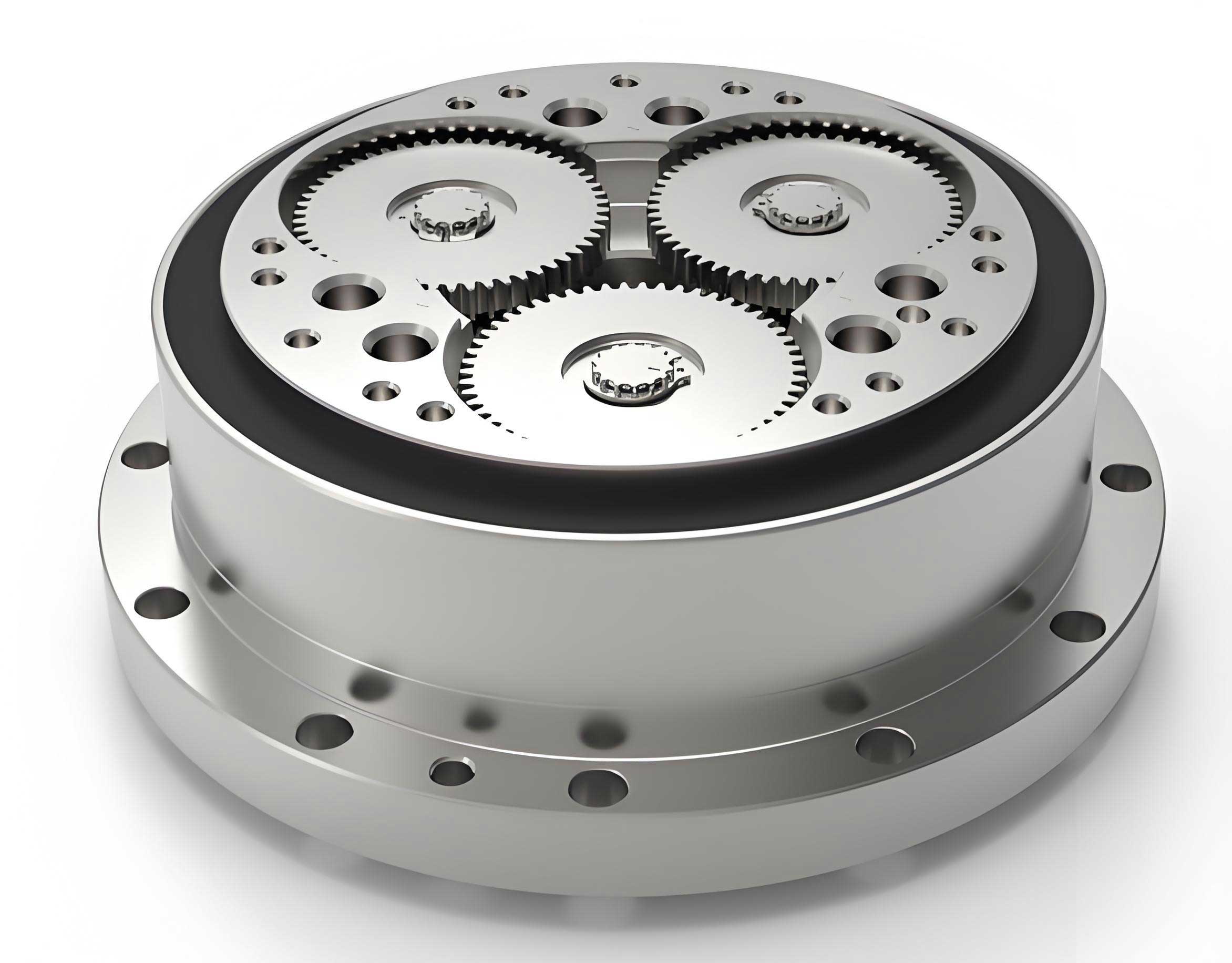
The kinematic structure of a typical dual-crank rotary vector reducer can be simplified. The system comprises an input sun gear (1), planetary gears (2) mounted on crankshafts, cycloidal gears (3), a stationary pinwheel ring (6) with needle rollers, and an output mechanism (5), often a W-output or flange. The two cycloidal gears are typically offset by 180° to balance inertial forces. Understanding the overall reduction ratio is fundamental to characterizing the rotary vector reducer’s performance.
1.1 Relative Velocity Method for Reduction Ratio
The total reduction ratio \( i \) is defined as the ratio of the input angular velocity \( \omega_1 \) to the output angular velocity \( \omega_5 \) ( \( i = \omega_1 / \omega_5 \) ). A relative motion analysis is applied at key interfaces.
The fundamental kinematic relationship from the cycloidal stage establishes that the absolute angular velocity of the cycloidal gear \( \omega_3 \) equals the output angular velocity \( \omega_5 \) due to the direct coupling via the W-output mechanism: \( \omega_3 = \omega_5 \).
Considering the velocity at the meshing point between the crankshaft pin and the cycloidal gear’s bore (point A in a typical analysis diagram), we have the velocity constraint:
$$ \omega_5 (b + c) + \omega_{2r5} \cdot b = -\omega_3 a $$
where:
\( \omega_{2r5} \) is the angular velocity of the crankshaft/planetary gear assembly (2) relative to the output carrier (5),
\( a \) is the eccentricity of the crankshaft,
\( b \) is the radius difference between the pinwheel and the cycloidal gear’s pitch circle,
\( c \) is a geometric dimension fulfilling \( a + b + c = R_6 \), the pinwheel center circle radius.
Simultaneously, the velocity at the meshing point between the sun gear and the planetary gear (point B) provides another constraint:
$$ \omega_5 R_1 – \omega_{2r5} R_2 = \omega_1 R_1 $$
where \( R_1 \) and \( R_2 \) are the pitch radii of the sun gear and planetary gear, respectively. These radii are directly related to their tooth numbers \( Z_1 \) and \( Z_2 \), and the common module \( m \): \( R_1 = mZ_1/2 \), \( R_2 = mZ_2/2 \).
Substituting \( \omega_3 = \omega_5 \) and the geometric relation \( b = R_6 – R_3 \) (where \( R_3 \) is the pitch radius of the cycloidal gear) into the equations and solving for the ratio \( \omega_1 / \omega_5 \) yields:
$$ \frac{\omega_1}{\omega_5} = 1 + \frac{R_2 R_6}{(R_6 – R_3) R_1} $$
Expressing the radii in terms of tooth numbers for the gear stage ( \( R_2/R_1 = Z_2/Z_1 \) ) and the cycloidal stage ( \( R_3/R_6 \approx Z_c / Z_p \) , where \( Z_c \) and \( Z_p \) are the number of lobes on the cycloidal disk and the number of pins in the pinwheel, respectively), we arrive at the comprehensive reduction ratio formula for the rotary vector reducer:
$$ i = \frac{\omega_1}{\omega_5} = 1 + \frac{Z_p \cdot Z_2}{Z_1 (Z_p – Z_c)} $$
For a common configuration like the RV-40E model with \( Z_1=10 \), \( Z_2=26 \), \( Z_p=40 \), and \( Z_c=39 \), the reduction ratio calculates to:
$$ i = 1 + \frac{40 \times 26}{10 \times (40 – 39)} = 1 + 104 = 105 $$
This high single-stage reduction ratio is a hallmark of the rotary vector reducer design.
2. Static Force Analysis of the Cycloidal-Pin Meshing
The second-stage cycloidal drive is the heart of the rotary vector reducer, responsible for the major portion of speed reduction and torque amplification. Accurate force analysis is critical for assessing stress, load distribution, and ultimately, the lifespan and reliability of the reducer.
2.1 Meshing Force Distribution with Profile Modification
In an ideal, unmodified cycloidal drive with perfect geometry, nearly half of the pins would simultaneously share the load. However, in practice, cycloidal gears are intentionally modified (via equidistant, offset, or combined profile shifting) to optimize backlash, lubrication, and load distribution. Without considering elastic deformations, these modifications result in only one or a few tooth pairs being in theoretical contact, with initial gaps \( \Delta(\varphi_i) \) present at other potential contact points.
The initial normal gap \( \Delta(\varphi_i) \) at the i-th pin position, defined by its angle \( \varphi_i \) relative to the line of centers, is a function of the modification parameters:
$$ \Delta(\varphi_i) = \Delta_r \left( \frac{1 – k \cos\varphi_i – \sqrt{1 – k^2} \sin\varphi_i}{\sqrt{1 + k^2 – 2k \cos\varphi_i}} \right) + \Delta_{rr} \left( 1 – \frac{\sin\varphi_i}{\sqrt{1 + k^2 – 2k \cos\varphi_i}} \right) $$
where:
\( k \) is the short width coefficient, \( k = e Z_p / r_z \),
\( e \) is the crankshaft eccentricity,
\( r_z \) is the pin circle radius,
\( \Delta_r \) is the offset (or “move distance”) modification,
\( \Delta_{rr} \) is the equidistant modification.
2.2 Elastic Deformation and Multi-Tooth Contact
Under operational load, elastic deformations of the components close these initial gaps, leading to multi-tooth contact. The total contact deformation \( \delta_i \) at the i-th pin consists of two parts in series: 1) the Hertzian contact deformation \( \omega_{1i} \) between the cycloidal gear lobe and the pin (roller), and 2) the contact deformation \( \omega_{2i} \) between the pin and the pinwheel housing bore (for designs without needle roller sleeves).
The general formula for contact deformation between two cylinders of length \( L \) under force \( F_i \) is given by:
$$ \omega = \frac{2F_i}{\pi L} \left[ \frac{1-\mu_1^2}{E_1} \left( \frac{1}{3} + \ln\frac{4R_1}{b} \right) + \frac{1-\mu_2^2}{E_2} \left( \frac{1}{3} + \ln\frac{4R_2}{b} \right) \right] $$
where \( E_1, E_2 \) are Young’s moduli, \( \mu_1, \mu_2 \) are Poisson’s ratios, \( R_1, R_2 \) are the contact radii, and \( b \) is the half-width of the contact area, calculable from Hertzian theory:
$$ b = 1.60 \sqrt{ \frac{F_i}{L} K_D \left( \frac{1-\mu_1^2}{E_1} + \frac{1-\mu_2^2}{E_2} \right) } $$
The equivalent radius of curvature \( K_D \) differs for each contact pair. For the convex-convex contact between the cycloid lobe (radius of curvature \( \rho_i \)) and the pin (radius \( r_{rp} \)):
$$ K_{D1} = \frac{2 \rho_i r_{rp}}{(\rho_i + r_{rp})}, \quad \text{where } \rho_i = \frac{(r_z + \Delta_r)(1+k^2-2k\cos\varphi_i)^{3/2}}{k(Z_p+1)\cos\varphi_i – (1+Z_p k^2)} + (r_{rp} + \Delta_{rr}) $$
For the convex-concave contact between the pin and the housing bore (radius \( r_p \)):
$$ K_{D2} = \frac{2 r_p r_{rp}}{(r_p – r_{rp})} $$
The total compliance at position \( i \) is \( C_i = (\omega_{1i} + \omega_{2i}) / F_i \). When the system is subjected to an output torque \( T \), shared by \( N \) cycloidal gears (typically \( N=2 \)), the torque per cycloid disk is \( T_c = T / N \). The load causes a slight rotational displacement \( \beta \) of the cycloidal disk. The normal elastic approach \( \delta_i \) at the i-th pin is geometrically related to \( \beta \):
$$ \delta_i = l_i \beta = \frac{l_i}{r’_c} \delta_{max} $$
where \( l_i \) is the moment arm from the cycloid center to the contact normal, \( l_i = r’_c \sin\varphi_i / \sqrt{1+k^2-2k\cos\varphi_i} \), \( r’_c = e Z_c \) is the cycloid generating circle radius, and \( \delta_{max} = l_{max} \beta \) is the maximum deformation at the most heavily loaded pin.
Contact occurs at pin \( i \) only if the elastic approach exceeds the initial gap: \( \delta_i > \Delta(\varphi_i) \). For contacting pins, the force is proportional to the net deformation:
$$ F_i = \frac{\delta_i – \Delta(\varphi_i)}{\delta_{max}} F_{max} $$
The forces must equilibrate the applied torque \( T_c \):
$$ T_c = \sum_{i \in S} F_i l_i = F_{max} \sum_{i \in S} \left( \frac{l_i}{r’_c} – \frac{\Delta(\varphi_i)}{\delta_{max}} \right) l_i $$
where \( S \) is the set of pins in contact. Since \( \delta_{max} \) itself depends on \( F_{max} \) through the deformation equations, an iterative solution is required. An initial estimate for \( F_{max} \) can be taken as the average of the theoretical values for the unmodified case and the single-point contact case:
$$ F_{max}^{(0)} = \frac{1}{2} \left( \frac{4 T_c k}{Z_c r_z} + \frac{T_c}{e Z_c} \right) $$
This value is used to calculate deformations, determine the contact set \( S \), and then solve for a new \( F_{max} \). The process iterates until convergence. The contact (Hertz) stress at each pin can then be evaluated:
$$ \sigma_{Hi} = 0.418 \sqrt{ \frac{F_i E_{eq}}{L \rho_{eqi}} } $$
where \( E_{eq} = 2E_1E_2/(E_1+E_2) \) is the equivalent modulus, and \( \rho_{eqi} = \rho_i r_{rp} / (\rho_i – r_{rp}) \) is the equivalent contact curvature radius.
2.3 Example Calculation for an RV-40E Model
Applying the above methodology to a typical rotary vector reducer (RV-40E) with the parameters below yields the meshing force and stress distribution. Key parameters include: Pin circle radius \( r_z = 64 \text{ mm} \), Pin radius \( r_{rp} = 3 \text{ mm} \), Housing bore radius \( r_p = 70 \text{ mm} \), Eccentricity \( e = 1.3 \text{ mm} \), Number of pins \( Z_p = 40 \), Number of cycloid lobes \( Z_c = 39 \), Cycloid disk thickness \( L = 8.86 \text{ mm} \), Offset modification \( \Delta_r = +0.008 \text{ mm} \), Equidistant modification \( \Delta_{rr} = -0.002 \text{ mm} \), Output torque \( T = 572 \text{ N·m} \), Torque per cycloid \( T_c = 286 \text{ N·m} \).
The iterative solution reveals a multi-tooth contact pattern. The calculated maximum meshing force \( F_{max} \) is approximately 1191 N. The contact forces and corresponding Hertz stresses for the engaged pins are summarized in Table 1.
| Pin Index (i) | Angle \( \varphi_i \) (deg) | Meshing Force \( F_i \) (N) | Contact Stress \( \sigma_{Hi} \) (MPa) |
|---|---|---|---|
| 2 | 18 | 762.7 | 935.5 |
| 3 | 27 | 1107.7 | 1147.2 |
| 4 | 36 | 1190.8 | 1276.9 |
| 5 | 45 | 1151.5 | 1320.1 |
| 6 | 54 | 1046.2 | 1323.0 |
| 7 | 63 | 901.2 | 1290.8 |
| 8 | 72 | 730.5 | 1223.2 |
| 9 | 81 | 542.6 | 1114.4 |
| 10 | 90 | 343.1 | 948.2 |
| 11 | 99 | 135.9 | 657.3 |
The resultant force components on a single cycloidal disk from all contacting pins are obtained by vector summation:
$$ F_{Rx} = \sum_{i \in S} F_i \cos\beta_i, \quad F_{Ry} = \sum_{i \in S} F_i \sin\beta_i $$
where \( \beta_i = \arctan\left( (\cos\varphi_i – k) / \sin\varphi_i \right) \) is the pressure angle. For this example, \( F_{Rx} \approx 7422 \text{ N} \) and \( F_{Ry} \approx 1246 \text{ N} \).
3. Parametric Sensitivity Analysis Using the Osculating Value Method
The performance and load capacity of a rotary vector reducer are sensitive to numerous geometric and material parameters. To guide optimization, it is crucial to rank these parameters based on their influence on critical performance metrics, such as meshing forces and stresses. The osculating value method is a multi-criteria decision-making technique suitable for such ranking.
3.1 Methodology of the Osculating Value Method
The osculating value method evaluates and ranks different alternatives (here, design parameters) based on their relative closeness to an idealized “best point” and distance from an idealized “worst point” across multiple evaluation indices. The procedure is as follows:
1. Construct the Decision Matrix: For \( n \) parameters to be evaluated (alternatives) and \( m \) evaluation indices, form an \( n \times m \) matrix \( X = (x_{ij}) \), where \( x_{ij} \) is the value of the j-th index for the i-th parameter.
2. Normalize the Decision Matrix: Convert all indices to dimensionless, comparable values. For benefit-type indices (where larger is better) and cost-type indices (where smaller is better), different normalization formulas are used. A common vector normalization is:
$$ r_{ij} = \frac{x_{ij}}{\sqrt{\sum_{i=1}^{n} x_{ij}^2}} $$
resulting in the normalized matrix \( R = (r_{ij}) \).
3. Determine the Best and Worst Reference Points: The best point \( G \) and the worst point \( B \) are virtual alternatives composed of the best and worst values for each index across all parameters, respectively.
$$ G = (g_1, g_2, …, g_m), \quad g_j = \begin{cases} \max_i(r_{ij}), & \text{if benefit index} \\ \min_i(r_{ij}), & \text{if cost index} \end{cases} $$
$$ B = (b_1, b_2, …, b_m), \quad b_j = \begin{cases} \min_i(r_{ij}), & \text{if benefit index} \\ \max_i(r_{ij}), & \text{if cost index} \end{cases} $$
4. Calculate Distances: Compute the Euclidean distance from each parameter \( i \) to the best point \( (d_i^G) \) and to the worst point \( (d_i^B) \):
$$ d_i^G = \sqrt{\sum_{j=1}^{m} (r_{ij} – g_j)^2}, \quad d_i^B = \sqrt{\sum_{j=1}^{m} (r_{ij} – b_j)^2} $$
5. Compute the Osculating Value \( C_i \): The osculating value for parameter \( i \) is defined as:
$$ C_i = \frac{d_i^G}{\min_i(d_i^G)} – \frac{d_i^B}{\max_i(d_i^B)} $$
A smaller \( C_i \) indicates that the parameter is closer to the best point and farther from the worst point across all considered indices, implying a greater (or more favorable) influence on the system according to the chosen criteria.
3.2 Application to Rotary Vector Reducer Parameters
We consider five key design parameters of the rotary vector reducer for sensitivity analysis concerning their impact on the transmission force characteristics: Pin radius \( (r_{rp}) \), Offset modification \( (\Delta_r) \), Equidistant modification \( (\Delta_{rr}) \), Cycloid disk thickness \( (L) \), and Crankshaft eccentricity \( (e) \). Five evaluation indices are chosen:
- Change in X-Force (\( \Delta F_x \)): The absolute change in the resultant force component \( F_{Rx} \) when the parameter is perturbed by a small, fixed amount (e.g., +0.001 mm). A larger change indicates higher sensitivity of load distribution.
- Change in Y-Force (\( \Delta F_y \)): The absolute change in the resultant force component \( F_{Ry} \).
- Nominal Parameter Value: The typical magnitude of the parameter. This is a cost index; a smaller nominal value may imply tighter manufacturing tolerances are needed for the same absolute change.
- Material Elastic Modulus (E): The typical Young’s modulus of the component. A higher modulus generally reduces elastic deformation.
- Manufacturing Difficulty Score: A qualitative score (e.g., 0.1 to 0.5) representing the relative difficulty of achieving precision in that parameter, with a higher score indicating greater difficulty (cost index).
Based on the analysis of the RV-40E model and general engineering knowledge, a hypothetical but representative decision matrix is constructed (Table 2).
| Parameter | \( \Delta F_x \) (N) | \( \Delta F_y \) (N) | Nominal Value (mm) | Elastic Modulus (GPa) | Difficulty Score |
|---|---|---|---|---|---|
| Pin Radius \( (r_{rp}) \) | 8.5 | 0.15 | 3.000 | 208 | 0.15 |
| Offset Mod. \( (\Delta_r) \) | 350.4 | -7.7 | 0.008 | 207 | 0.25 |
| Equidistant Mod. \( (\Delta_{rr}) \) | -298.2 | -3.7 | 0.002 | 207 | 0.25 |
| Cycloid Thickness \( (L) \) | 0.1 | 0.01 | 8.860 | 207 | 0.15 |
| Eccentricity \( (e) \) | -9.0 | 1.6 | 1.300 | 207 | 0.20 |
*Note: \( \Delta F_x, \Delta F_y \) are illustrative values representing sensitivity to a +0.001 mm perturbation. Negative values indicate a decrease in force.
Following the osculating value method steps (normalization, determination of best/worst points, distance calculation) yields the final osculating values \( C_i \) and the corresponding ranking, as shown in Table 3.
| Parameter | Osculating Value \( C_i \) | Rank (1=Most Influential) |
|---|---|---|
| Cycloid Disk Thickness \( (L) \) | 0.000 | 1 |
| Pin Radius \( (r_{rp}) \) | 2.663 | 2 |
| Crankshaft Eccentricity \( (e) \) | 3.499 | 3 |
| Offset Modification \( (\Delta_r) \) | 4.040 | 4 |
| Equidistant Modification \( (\Delta_{rr}) \) | 4.050 | 5 |
3.3 Interpretation and Design Implications
The osculating value analysis provides a multi-faceted ranking. The cycloid disk thickness \( (L) \) emerges as the most influential parameter according to this combined set of criteria. While a small geometric perturbation in \( L \) causes minimal immediate change in force components \( (\Delta F_x, \Delta F_y) \), its large nominal value directly and significantly affects the contact compliance (through the contact length in Hertz formulas), the bending stiffness of the cycloid disk, and the overall load capacity. Its manufacturing difficulty is also relatively low (machining a precise thickness). Therefore, it is a primary variable for optimization in a rotary vector reducer design.
The pin radius \( (r_{rp}) \) and the crankshaft eccentricity \( (e) \) rank second and third, respectively. Both have moderate to high influence on force sensitivity and are key geometric parameters defining the cycloidal mesh geometry (short width coefficient \( k \)) and the reduction ratio. The modification parameters \( (\Delta_r, \Delta_{rr}) \), while crucial for fine-tuning backlash and optimizing load distribution under deformation, show a lower composite influence score in this particular assessment, partly due to their very small nominal values which make proportional control easier, but also because their effects are highly nonlinear and interdependent.
This analytical conclusion strongly suggests that in structural optimization of a rotary vector reducer, priority should be given to selecting the cycloid disk thickness, the crankshaft eccentricity, and the pin/roller radius as primary design variables. Optimizing these parameters first will have the most substantial impact on improving the torque density, load distribution, and overall mechanical efficiency of the transmission.
4. Conclusion
This comprehensive analysis has elucidated the core operational principles of the rotary vector reducer. The kinematic derivation using the relative velocity method provides a clear and rigorous path to understanding its characteristically high reduction ratio. The detailed static force analysis model for the cycloidal-pin mesh, accounting for intentional profile modifications and elastic deformations, forms the foundation for accurate load distribution and stress prediction, which are paramount for reliability assessment and design validation.
Furthermore, the application of the osculating value method offers a systematic, multi-criteria framework for evaluating the relative influence of key design parameters on the force transmission characteristics. The outcome identifies the cycloid disk thickness, crankshaft eccentricity, and pin radius as the parameters most closely tied to the transmission force behavior. These findings provide valuable, prioritized guidance for engineers undertaking the design optimization of high-performance rotary vector reducers, enabling focused efforts on the variables that promise the greatest return in terms of enhanced load capacity, efficiency, and compactness. The methodologies presented herein contribute to the deeper understanding and advanced development of this critical component in precision motion control systems.