
In the field of industrial robotics, the rotary vector reducer plays a critical role in providing high precision, high torque, and compact motion control. As a key component, the cycloidal gear within the rotary vector reducer requires exceptional accuracy and surface finish to ensure smooth operation, minimal backlash, and long service life. Traditional gear grinding methods, such as generating grinding, often fall short in terms of efficiency and flexibility, especially when dealing with complex tooth profile modifications. This has led to the adoption of form grinding, where the grinding wheel’s axial profile matches the tooth slot shape exactly, enabling full-depth engagement and significantly improving machining efficiency. In this article, I will explore the form grinding process for cycloidal gears in rotary vector reducers, focusing on wheel profile modification, mathematical modeling, and simulation techniques. I will delve into tooth profile modification mechanisms, the derivation of form grinding equations, wheel widening theory, diamond dressing trajectory calculations, and the development of simulation software. Throughout, I will emphasize the importance of the rotary vector reducer in robotic applications and how advanced form grinding can enhance its performance.
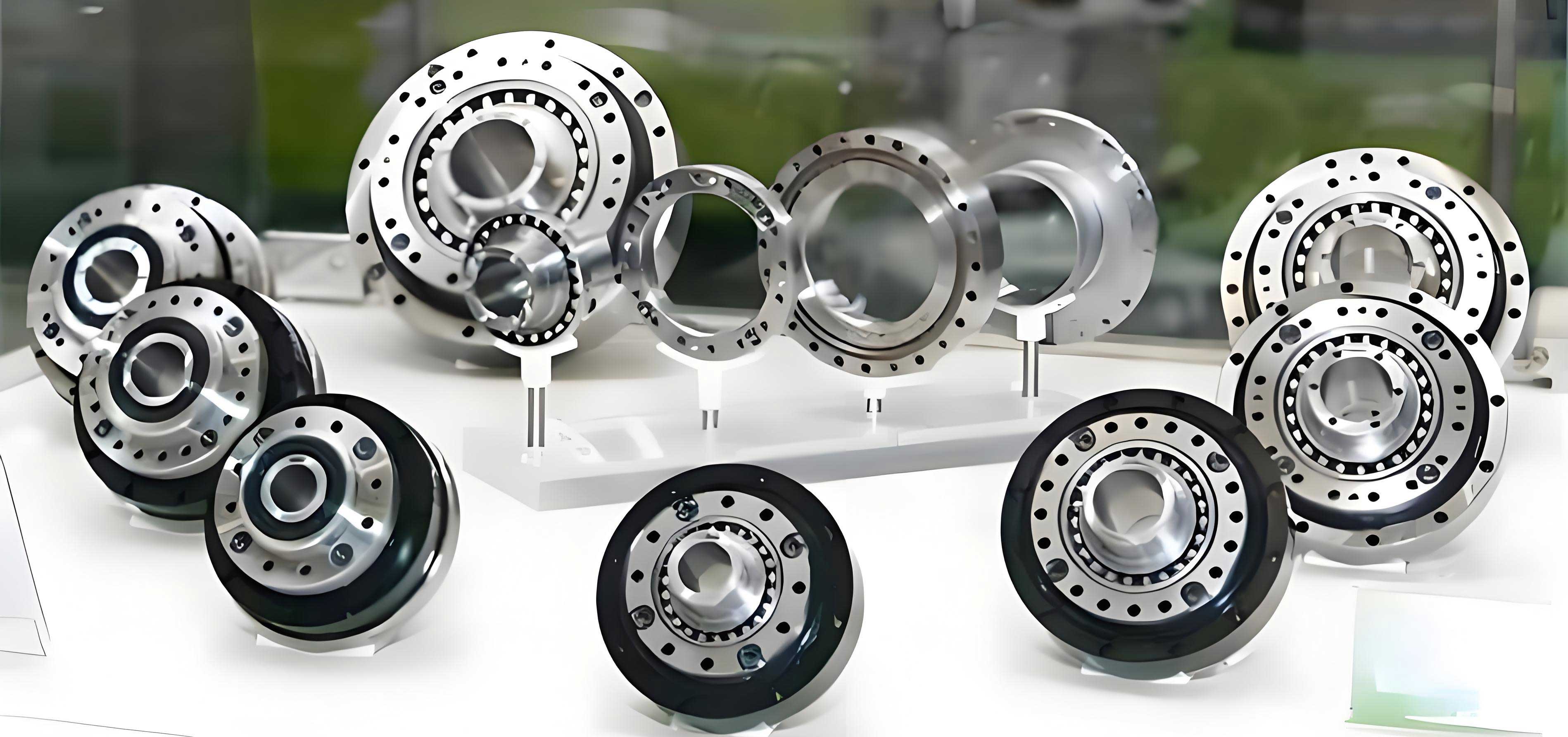
The rotary vector reducer, commonly known as the RV reducer, is a precision speed reducer used extensively in robotics, machine tools, and aerospace. Its compact design and high load-carrying capacity stem from a two-stage reduction mechanism that includes a cycloidal drive. The cycloidal gear, with its epitrochoidal tooth profile, meshes with needle bearings to provide high reduction ratios and excellent torsional stiffness. However, to accommodate manufacturing tolerances, ensure proper lubrication, and minimize backlash, the cycloidal tooth profile often requires modification. Traditional modification methods include equidistant and shift modifications, but recent advancements have introduced parabolic modification for optimal performance. In form grinding, the grinding wheel is dressed to mirror the modified tooth slot profile, allowing for efficient and precise gear finishing. This process is particularly advantageous for rotary vector reducers, where dual cycloidal gears are often ground simultaneously to guarantee identical tooth profiles for balanced operation.
Tooth profile modification for cycloidal gears in rotary vector reducers is essential to compensate for errors and improve meshing conditions. The most common methods are equidistant and shift modifications, often combined as “equidistant plus shift” modification. For instance, negative equidistant modification combined with positive shift modification is preferred in many rotary vector reducer applications because it reduces backlash and maintains a close approximation to the ideal profile. The mathematical representation of a modified cycloidal tooth profile can be derived from the standard epitrochoidal equation. Let the standard profile be defined by parameters such as the pinion radius \(R_z\), needle radius \(r_z\), eccentricity \(A\), tooth numbers \(z_a\) and \(z_b\), and the short width coefficient \(K_1\). The standard coordinates in the gear coordinate system are:
$$ X_2 = R_z \sin \phi – A \sin(z_b \phi) + r_z \frac{K_1 \sin(z_b \phi) – \sin \phi}{\sqrt{1 + K_1^2 – 2K_1 \cos(z_a \phi)}} $$
$$ Y_2 = R_z \cos \phi – A \cos(z_b \phi) – r_z \frac{-K_1 \cos(z_b \phi) + \cos \phi}{\sqrt{1 + K_1^2 – 2K_1 \cos(z_a \phi)}} $$
where \(\phi\) is the rotation angle parameter. For modification, an additional term \(\Delta L\) is introduced to represent the modification amount. In equidistant modification, \(\Delta L\) is constant, while in shift modification, it varies linearly. For parabolic modification, \(\Delta L\) is a function of the arc length from a reference point, often expressed as \(\Delta L = a \cdot (\sqrt{R_z^2 + r_b^2 – 2R_z r_b \cos(z_a \phi)} – L_0)^2\), where \(a\) is the modification coefficient and \(L_0\) is the reference length. This parabolic approach minimizes deviation in the primary working zone, making it ideal for high-precision rotary vector reducers. However, for practical grinding, the combined equidistant and shift modification is more feasible. The modified profile equation becomes:
$$ X_2 = R_z \sin \phi – A \sin(z_b \phi) + (r_z + \Delta L) \frac{K_1 \sin(z_b \phi) – \sin \phi}{\sqrt{1 + K_1^2 – 2K_1 \cos(z_a \phi)}} $$
$$ Y_2 = R_z \cos \phi – A \cos(z_b \phi) – (r_z + \Delta L) \frac{-K_1 \cos(z_b \phi) + \cos \phi}{\sqrt{1 + K_1^2 – 2K_1 \cos(z_a \phi)}} $$
where \(\Delta L\) can be a constant for equidistant modification or include a shift component. For rotary vector reducers, the choice of modification affects the transmission error, load distribution, and backlash, so it must be carefully optimized.
| Modification Type | Description | Advantages for Rotary Vector Reducer | Typical Application |
|---|---|---|---|
| Equidistant | Constant offset along tooth normal | Simple to implement, provides clearance | General-purpose reducers |
| Shift | Linear shift of tooth profile | Adjusts meshing position, reduces backlash | High-precision robotics |
| Parabolic | Non-linear modification based on arc length | Minimizes deviation in working zone, optimal for stiffness | Advanced rotary vector reducers |
| Combined (Equidistant + Shift) | Hybrid of constant and linear modifications | Balances clearance and precision, widely used | Industrial robot reducers |
Form grinding for cycloidal gears in rotary vector reducers involves creating a grinding wheel whose axial cross-section matches the tooth slot profile of the modified gear. To establish the mathematical model, I define two coordinate systems: the gear coordinate system \(O_2-X_2Y_2Z_2\) attached to the cycloidal gear, and the grinding wheel coordinate system \(O_G-X_GY_GZ_G\) attached to the wheel. The \(Z_2\)-axis aligns with the gear axis, and the \(X_G\)-axis aligns with the wheel axis. The distance between these axes is \(E = R_{ia} + R_G\), where \(R_{ia}\) is the gear root circle radius and \(R_G\) is the grinding wheel radius. The transformation matrix from the gear system to the wheel system, \(M_{G2}\), accounts for the relative positioning. For a point on the gear tooth surface represented as \(\mathbf{r}_2 = [X_2, Y_2, z_2, 1]^T\), the corresponding point in the wheel system is \(\mathbf{r}_G = M_{G2} \mathbf{r}_2\). The axial profile of the grinding wheel, which lies in the \(X_GY_G\)-plane, has coordinates:
$$ \begin{bmatrix} X_G \\ Y_G \end{bmatrix} = \begin{bmatrix} x_G \\ y_G \end{bmatrix} = \begin{bmatrix} X_2 \\ Y_2 – E \end{bmatrix} $$
where \(Y_G\) gives the wheel radius \(R_G\) at that axial position. By discretizing the modified tooth profile equation over the gear width, I can compute the wheel profile coordinates. This process is crucial for dressing the grinding wheel accurately to produce the desired tooth form in the rotary vector reducer.
One challenge in form grinding cycloidal gears for rotary vector reducers is ensuring continuity at the junctions between adjacent teeth, as the grinding is performed discretely for each tooth slot. To address this, wheel widening is employed, where the wheel profile is extended beyond the theoretical width to blend any step marks caused by indexing errors. The widened portion typically uses a circular arc as a transition curve, chosen based on the curvature of the tooth profile at the highest point of the slot. The curvature radius \(\rho\) at any point on the profile is given by:
$$ \rho = \frac{\left( \left( \frac{dX_2}{d\phi} \right)^2 + \left( \frac{dY_2}{d\phi} \right)^2 \right)^{3/2}}{\frac{dX_2}{d\phi} \cdot \frac{d^2 Y_2}{d\phi^2} – \frac{dY_2}{d\phi} \cdot \frac{d^2 X_2}{d\phi^2}} $$
At the point of curvature reversal (where the curvature changes sign), the radius is minimal and positive. By selecting an arc with radius equal to the curvature radius at the profile’s highest point, I can ensure a smooth transition. Let the wheel’s theoretical width be \(B\), and the widened width be \(b\). The transition arc, defined in a local coordinate system \(O_N-X_NY_N\), has the equation \(\mathbf{r}_N = [\rho_N \cos \theta, \rho_N \sin \theta, 0, 1]^T\) for \(0 \leq \theta \leq b/(2\rho_N)\). Transforming this to the gear system and then to the wheel system yields the widened wheel profile coordinates:
$$ \begin{bmatrix} X_G \\ Y_G \end{bmatrix} = \begin{bmatrix} -\rho_N \sin(\pi/z_a) \cos \theta + \rho_N \cos(\pi/z_a) \sin \theta + X_2^{(O_N)} \\ -\rho_N \cos(\pi/z_a) \cos \theta + \rho_N \sin(\pi/z_a) \sin \theta + Y_2^{(O_N)} – E \end{bmatrix} $$
where \(X_2^{(O_N)}\) and \(Y_2^{(O_N)}\) are the coordinates of the arc center in the gear system. This widening technique is vital for producing seamless tooth profiles in rotary vector reducers, enhancing their smooth operation and durability.
After determining the grinding wheel profile, the next step is dressing the wheel using a diamond roller. The dressing trajectory is the offset curve of the wheel profile, based on the principle of equidistant curves. For a given wheel profile point \(\mathbf{r}_G\), the corresponding diamond roller center position \(\mathbf{r}_R\) is given by:
$$ \mathbf{r}_R = \mathbf{r}_G + R_d \cdot \mathbf{n} $$
where \(R_d\) is the diamond roller radius and \(\mathbf{n}\) is the unit normal vector to the wheel profile. The normal vector can be computed from the profile derivatives. If the wheel profile is parameterized by \(u\), with coordinates \((X_G(u), Y_G(u))\), then the tangent vector is \(\mathbf{t} = (dX_G/du, dY_G/du)\), and the unit normal is \(\mathbf{n} = (-dY_G/du, dX_G/du) / \|\mathbf{t}\|\). Substituting into the offset equation yields the dressing trajectory coordinates:
$$ X_R = X_G – R_d \cdot \frac{dY_G/du}{\sqrt{(dX_G/du)^2 + (dY_G/du)^2}} $$
$$ Y_R = Y_G + R_d \cdot \frac{dX_G/du}{\sqrt{(dX_G/du)^2 + (dY_G/du)^2}} $$
This trajectory is then used to program the CNC dressing system on the form grinding machine. Accurate calculation of this path is essential for achieving the precise wheel profile needed for high-quality cycloidal gears in rotary vector reducers.
To facilitate the design and verification process, I developed a simulation software based on Matlab. This software implements the mathematical models discussed above and provides a user-friendly interface for inputting gear parameters, modification coefficients, and wheel specifications. The core functionalities include: (1) computation of cycloidal tooth profiles for standard and modified cases, (2) calculation of grinding wheel axial profiles, (3) determination of wheel widening parameters, (4) generation of diamond dressing trajectories, and (5) graphical simulation of the grinding and dressing processes. The software outputs numerical data and plots, such as wheel profile comparisons and dressing paths, which can be directly used in CNC programming for rotary vector reducer manufacturing. Below is a summary of typical input parameters for the software, relevant to rotary vector reducer applications:
| Parameter | Symbol | Typical Value Range | Description |
|---|---|---|---|
| Gear Tooth Number | \(z_a\) | 15-41 (odd) | Number of teeth on cycloidal gear |
| Pinion Tooth Number | \(z_b\) | \(z_a + 1\) | Number of needle bearings |
| Pinion Radius | \(R_z\) | 50-150 mm | Radius of pin circle |
| Needle Radius | \(r_z\) | 3-10 mm | Radius of needle bearings |
| Eccentricity | \(A\) | 1-5 mm | Eccentric distance in cycloidal drive |
| Short Width Coefficient | \(K_1\) | 0.6-0.9 | Parameter defining tooth shortening |
| Equidistant Modification | \(\Delta r\) | ±0.01-0.1 mm | Constant offset for modification |
| Shift Modification | \(\Delta s\) | ±0.01-0.1 mm | Linear shift amount |
| Grinding Wheel Radius | \(R_G\) | 100-300 mm | Radius of form grinding wheel |
| Diamond Roller Radius | \(R_d\) | 5-20 mm | Radius of dressing tool |
The software operates by first calculating the discrete points on the modified tooth profile using the equations provided earlier. For instance, for parabolic modification, the modification amount \(\Delta L\) is computed as \(a \cdot (\sqrt{R_z^2 + r_b^2 – 2R_z r_b \cos(z_a \phi)} – L_0)^2\), where \(a\) and \(L_0\) are user-defined. The profile points are then transformed to the wheel coordinate system to obtain the axial profile. The wheel widening module adds the transition arc based on curvature analysis. Finally, the dressing trajectory is derived using the offset curve method. All computations are performed with high numerical precision to ensure accuracy for rotary vector reducer components.
In practical applications for rotary vector reducers, the form grinding process involves a five-axis CNC machine with linear axes (X, Y, Z) and rotational axes (workpiece rotation and wheel rotation). The grinding cycle includes: positioning the wheel relative to the gear, feeding radially along Y-axis, oscillating axially along Z-axis to grind the full tooth slot width, retracting, indexing the workpiece by \(2\pi/z_a\), and repeating for all teeth. The dressing cycle uses the X and Z axes to move the diamond roller along the computed trajectory, sculpting the wheel profile. This setup allows for efficient grinding of dual cycloidal gears simultaneously, which is common in rotary vector reducers to ensure phase alignment and load sharing.
The advantages of form grinding for cycloidal gears in rotary vector reducers are manifold. Compared to generating grinding, it offers higher material removal rates due to full-depth engagement, reducing machining time. The ability to incorporate complex modifications directly into the wheel profile enhances flexibility and precision. Moreover, with deep-cut slow-feed grinding and effective cooling, the risk of tooth surface burn is minimized, making it suitable for hard finishing of hardened gears. The rotary vector reducer benefits from this through improved gear accuracy, leading to lower noise, higher efficiency, and longer lifespan in robotic joints.
To illustrate the mathematical depth, let me expand on the coordinate transformations. The transformation matrix \(M_{G2}\) from the gear system to the wheel system involves a translation and rotation. Assuming the gear axis is parallel to the Z2-axis and the wheel axis is parallel to the XG-axis, with a center distance E, the matrix can be expressed as:
$$ M_{G2} = \begin{bmatrix}
0 & -1 & 0 & 0 \\
1 & 0 & 0 & -E \\
0 & 0 & 1 & 0 \\
0 & 0 & 0 & 1
\end{bmatrix} $$
This assumes the gear and wheel axes are perpendicular and offset. For a point on the gear, \(\mathbf{r}_2 = [X_2, Y_2, z_2, 1]^T\), the transformation gives \(\mathbf{r}_G = [x_G, y_G, z_G, 1]^T = [-Y_2, X_2 – E, z_2, 1]^T\). However, in the axial profile, we only consider \(x_G\) and \(y_G\), as \(z_G\) corresponds to the wheel width direction. Thus, the axial profile coordinates are \(X_G = x_G = -Y_2\) and \(Y_G = y_G = X_2 – E\). This matches the earlier simplified equation when accounting for coordinate orientation differences. In practice, for rotary vector reducer gears, the profile is symmetric, so only half may be computed and mirrored.
Furthermore, the curvature analysis for wheel widening can be detailed. The curvature \(\kappa\) is the reciprocal of the radius, \(\kappa = 1/\rho\). For a parametric curve \((X(\phi), Y(\phi))\), the curvature is given by:
$$ \kappa = \frac{X’ Y” – Y’ X”}{(X’^2 + Y’^2)^{3/2}} $$
where primes denote derivatives with respect to \(\phi\). By evaluating this at the tooth slot’s highest point, I find the curvature radius for the transition arc. This point often corresponds to \(\phi = \pi/z_a\), where the profile has local extremum. The transition arc is then designed to match this curvature, ensuring G2 continuity (same curvature) at the junction, which is critical for smooth meshing in rotary vector reducers.
In terms of software implementation, the Matlab code uses object-oriented programming to handle different modification types. The main classes include CycloidalGear, GrindingWheel, DressingTool, and SimulationEngine. The software allows users to select modification methods: standard, equidistant, shift, combined, or parabolic. For parabolic modification, the user inputs coefficients \(a\) and \(L_0\), and the software solves for the profile iteratively to minimize transmission error. The output includes ASCII files of dressing coordinates that can be imported into CNC machines, as well as graphical plots like the one below (simulated in software):
Simulation results show that for a typical rotary vector reducer with \(z_a = 31\), \(z_b = 32\), \(R_z = 100\) mm, \(r_z = 6\) mm, \(A = 2\) mm, and \(K_1 = 0.8\), the form grinding wheel profile for negative equidistant (\(\Delta r = -0.05\) mm) and positive shift (\(\Delta s = +0.03\) mm) modification has a maximum deviation of 0.002 mm from the ideal profile. The dressing trajectory comprises over 10,000 points for high accuracy. The software also simulates the grinding process, predicting surface finish and potential errors due to machine kinematics.
Another aspect is the thermal management during grinding of rotary vector reducer gears. Since form grinding involves large contact areas, heat generation can be significant. However, with modern CNC machines equipped with high-pressure coolant systems, the wheel and workpiece are kept at stable temperatures, preserving gear accuracy. The software includes a thermal module to estimate temperature rise based on grinding parameters like feed rate, depth of cut, and coolant flow, but that is beyond the scope of this article.
To conclude, form grinding wheel profile modification for cycloidal gears in rotary vector reducers is a sophisticated process that integrates advanced mathematics, precision engineering, and software simulation. By deriving the modified tooth profile equations, calculating the corresponding grinding wheel axial profile, implementing wheel widening for continuity, and computing the diamond dressing trajectory, I can achieve high-precision gear finishing. The developed Matlab-based software streamlines this process, enabling efficient design and verification for various modification strategies. This advancement supports the manufacturing of high-performance rotary vector reducers, which are essential for modern robotics and automation. Future work may involve real-time adaptive control of the grinding process based on in-process measurements, further enhancing the quality of rotary vector reducers.
In summary, the key equations for form grinding cycloidal gears in rotary vector reducers are consolidated below:
$$ \text{Modified Tooth Profile: } \begin{cases} X_2 = R_z \sin \phi – A \sin(z_b \phi) + (r_z + \Delta L) \frac{K_1 \sin(z_b \phi) – \sin \phi}{\sqrt{1 + K_1^2 – 2K_1 \cos(z_a \phi)}} \\ Y_2 = R_z \cos \phi – A \cos(z_b \phi) – (r_z + \Delta L) \frac{-K_1 \cos(z_b \phi) + \cos \phi}{\sqrt{1 + K_1^2 – 2K_1 \cos(z_a \phi)}} \end{cases} $$
$$ \text{Wheel Axial Profile: } \begin{bmatrix} X_G \\ Y_G \end{bmatrix} = \begin{bmatrix} X_2 \\ Y_2 – E \end{bmatrix} $$
$$ \text{Wheel Widening Arc: } \mathbf{r}_N = [\rho_N \cos \theta, \rho_N \sin \theta, 0, 1]^T $$
$$ \text{Dressing Trajectory: } \mathbf{r}_R = \mathbf{r}_G + R_d \cdot \mathbf{n} $$
These formulas, along with the simulation tools, provide a comprehensive framework for optimizing the form grinding of cycloidal gears in rotary vector reducers, ensuring they meet the stringent demands of robotic applications.