
In the field of precision robotics and industrial automation, the rotary vector reducer has emerged as a critical component due to its compact design, high torque density, and large reduction ratios. As a researcher focused on mechanical dynamics, I have extensively studied the dynamic characteristics of these reducers, particularly their torsional vibration behavior. Torsional vibration, often induced by rapid stops or reciprocating motions in robotic arms, can significantly impact the performance and longevity of the rotary vector reducer. Therefore, understanding its natural frequencies, especially the first-order natural frequency, and identifying the primary influencing factors are essential for optimal design and application. This article presents a comprehensive analysis based on a lumped-parameter dynamic model, incorporating often-overlooked elements such as bearing stiffness, and validates the findings through experimental means.
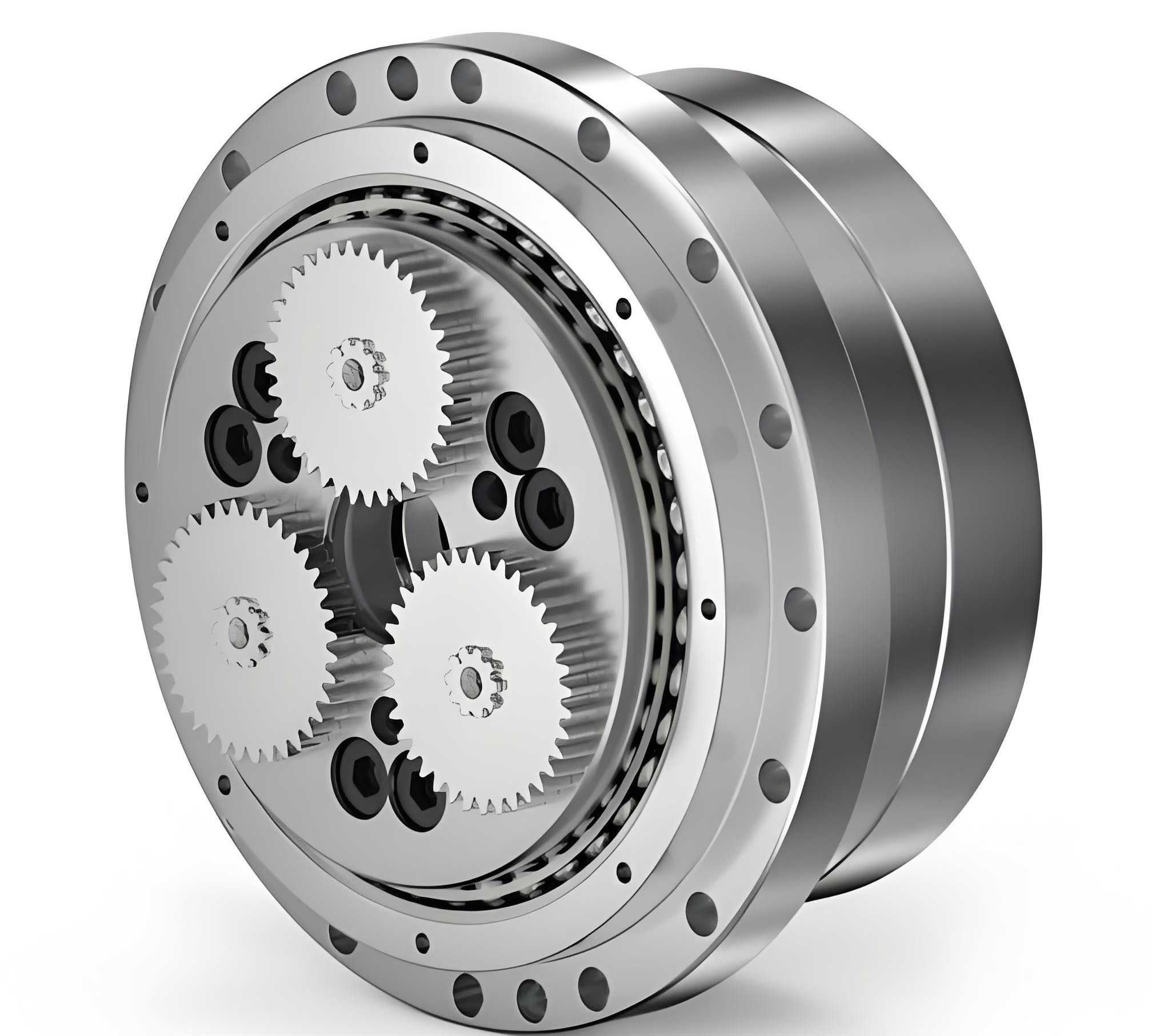
The rotary vector reducer, often abbreviated as RV reducer, is a sophisticated transmission system that evolved from cycloidal drive mechanisms. It typically consists of a two-stage reduction: the first stage involves a planetary gear train with a sun gear and planetary gears, and the second stage employs a cycloidal disc and pin gear arrangement. This combination allows the rotary vector reducer to achieve high reduction ratios in a relatively small envelope, making it ideal for applications like robotic joints where space and weight are constrained. However, the dynamic interactions within this complex system, particularly under transient loads, can lead to torsional vibrations that may cause noise, fatigue, or even failure. My investigation aims to model these vibrations accurately and pinpoint the most critical parameters affecting the system’s fundamental natural frequency.
To begin, it is crucial to understand the kinematic relationships within the rotary vector reducer. The overall speed reduction is derived from the combined effects of the planetary and cycloidal stages. Using the standard method for planetary trains, the speed ratio when the carrier (planet carrier) is fixed can be expressed. Let $\omega_s$, $\omega_p$, and $\omega_H$ denote the angular velocities of the sun gear, planetary gear, and carrier, respectively. The gear teeth numbers are $z_s$ for the sun gear and $z_p$ for the planetary gear. The transmission ratio for the first stage, assuming the carrier is fixed, is:
$$ i^{H}_{sp} = \frac{\omega_s – \omega_H}{\omega_p – \omega_H} = -\frac{z_p}{z_s} $$
For the second stage, the cycloidal-pin engagement, with the planetary gear fixed (i.e., the crank shaft fixed relative to the planetary gear), the ratio involves the cycloidal disc and the pin gear. Let $\omega_c$ and $\omega_r$ be the angular velocities of the cycloidal disc and pin gear, respectively, with teeth numbers $z_c$ and $z_r$. The relationship is:
$$ i^{p}_{cr} = \frac{\omega_c – \omega_p}{\omega_r – \omega_p} = \frac{z_r}{z_c} $$
In a standard rotary vector reducer, the pin gear is stationary ($\omega_r = 0$), and the cycloidal disc rotates at the same speed as the carrier ($\omega_c = \omega_H$). Furthermore, the tooth difference is typically one: $z_c = z_r – 1$. Combining these equations, the overall speed ratio between the sun gear (input) and the carrier (output) can be derived. The ratio between the planetary gear and sun gear is:
$$ i_{ps} = \frac{\omega_p}{\omega_s} = -\frac{z_s z_c}{z_s + z_r z_p} $$
And the ratio between the carrier and sun gear is:
$$ i_{Hs} = \frac{\omega_H}{\omega_s} = \frac{1}{1 + (z_c + 1) \frac{z_p}{z_s}} $$
These ratios are fundamental for later dynamic parameter equivalencing. For instance, in a common rotary vector reducer model like RV-6A, with $z_s=10$, $z_p=34$, $z_c=29$, and $z_r=30$, the reduction ratio $i_{Hs}$ is approximately 1/103, indicating a high reduction capability characteristic of the rotary vector reducer.
Moving to the dynamic modeling, I adopted a lumped-parameter approach to construct a pure torsional vibration model for the rotary vector reducer. This method simplifies the distributed system into discrete inertia elements connected by stiffness elements, focusing solely on rotational degrees of freedom. The model is based on several assumptions to maintain tractability while capturing essential dynamics. First, due to symmetry, the two crank shafts are assumed to move identically in phase and magnitude, allowing treatment as a single equivalent component. Second, the bending stiffness of the crank shaft is considered high relative to bearing stiffness, so bending deformations are neglected—a valid assumption given the short distances between bearing points. The main components are lumped as follows: the input gear shaft, planetary gears, crank shaft, cycloidal discs, and the carrier along with its load. Each is represented as an inertia disk, and the connecting stiffnesses include gear mesh stiffnesses, shaft torsional stiffnesses, and crucially, bearing radial stiffnesses.
The equivalent inertia and stiffness parameters are calculated by referring all elements to the input shaft (sun gear) based on energy equivalence principles. For kinetic energy, the equivalent moment of inertia $J_e^i$ for component $i$ is:
$$ J_e^i = J_i \left( \frac{\omega_i}{\omega_s} \right)^2 + m_i \left( \frac{v_i}{\omega_s} \right)^2 $$
where $J_i$ is the actual moment of inertia, $m_i$ is mass, $\omega_i$ is angular velocity, and $v_i$ is translational velocity of the center of mass. For symmetric parts like the two planetary gears, crank shafts, and cycloidal discs, the contributions are doubled. For example, for the planetary gears ($i=p$), with $v_p = r_b \omega_H$ where $r_b$ is the radius to the crank shaft axis on the carrier, and using the speed ratios $i_{ps}$ and $i_{Hs}$, the equivalent inertia becomes:
$$ J_e^p = 2 J_p i_{ps}^2 + 2 m_p r_b^2 i_{Hs}^2 $$
Similarly, for the crank shaft ($i=b$):
$$ J_e^b = 2 J_b i_{ps}^2 + 2 m_b r_b^2 i_{Hs}^2 $$
For the cycloidal discs ($i=c$), noting that $\omega_c = \omega_H$ and $v_c = a \omega_p$ where $a$ is the crank eccentricity:
$$ J_e^c = 2 J_c i_{Hs}^2 + 2 m_c a^2 i_{ps}^2 $$
And for the carrier including load ($i=H$):
$$ J_e^H = J_H i_{Hs}^2 $$
Potential energy equivalence is used for stiffness parameters. The equivalent torsional stiffness $k_e$ for each elastic element is derived from the condition that the strain energy remains invariant when referred to the input shaft. For instance, the sun-planet mesh stiffness $k_{sp}$ (in N/m) is converted to an equivalent torsional stiffness at the sun gear:
$$ k_e^{sp} = 2 k_{sp} r_s^2 $$
where $r_s$ is the base radius of the sun gear. The factor 2 accounts for two meshing points. The torsional stiffness of the crank shaft $k_b$ (in N·m/rad) becomes:
$$ k_e^{b} = 2 k_b i_{bs}^2 $$
with $i_{bs} = i_{ps}$. The bearing stiffnesses are critical. The radial stiffness of the bearings supporting the cycloidal discs on the crank pins, $k_{cb}$ (in N/m), contributes to torsional deformation via the eccentricity $a$:
$$ k_e^{cb} = 2 k_{cb} a^2 i_{bs}^2 $$
The cycloidal-pin mesh has both torsional and translational components. The torsional mesh stiffness $k_{cr}$ (in N·m/rad) and the tangential stiffness $k’_{cr}$ (in N/m) derived from the mesh stiffness per unit length and the pressure angle $\alpha$ are combined:
$$ k_e^{cr} = 2 k_{cr} i_{cs}^2 + 2 k’_{cr} a^2 i_{bs}^2 $$
where $i_{cs} = i_{Hs}$, and $k’_{cr} = \frac{k_{cr}}{r_c} \cos \alpha$ with $r_c$ as the fixed circle radius of the cycloidal disc. Finally, the radial stiffness of the bearings on the carrier, $k_{Hb}$ (in N/m), which supports the crank shafts, is equivalenced as:
$$ k_e^{Hb} = k_{Hb} r_b^2 i_{Hs}^2 $$
These equivalent parameters form a 5-degree-of-freedom torsional model, with generalized coordinates being the angular displacements of the sun gear $\theta_s$, equivalent planetary gear $\theta_p^e$, equivalent crank shaft $\theta_b^e$, equivalent cycloidal disc $\theta_c^e$, and equivalent carrier $\theta_H^e$, all referred to the input axis. The free vibration equation is:
$$ \mathbf{J} \ddot{\boldsymbol{\theta}} + \mathbf{K} \boldsymbol{\theta} = \mathbf{0} $$
where $\mathbf{J}$ is the diagonal inertia matrix and $\mathbf{K}$ is the stiffness matrix. The stiffness matrix $\mathbf{K}$ includes the input shaft torsional stiffness $k_I$ and all equivalent stiffnesses. Since gear mesh stiffnesses vary with time, for fundamental natural frequency calculation, average values over a cycle are used, making $\mathbf{K}$ constant. The explicit form of $\mathbf{K}$ for the rotary vector reducer model is:
$$ \mathbf{K} = \begin{bmatrix}
k_I + k_e^{sp} & -k_e^{sp} & 0 & 0 & 0 \\
-k_e^{sp} & k_e^{sp} + k_e^{b} & -k_e^{b} & 0 & 0 \\
0 & -k_e^{b} & k_e^{b} + k_e^{cb} + k_e^{Hb} & -k_e^{cb} & -k_e^{Hb} \\
0 & 0 & -k_e^{cb} & k_e^{cr} + k_e^{cb} & 0 \\
0 & 0 & -k_e^{Hb} & 0 & k_e^{Hb}
\end{bmatrix} $$
And the inertia matrix $\mathbf{J}$ is:
$$ \mathbf{J} = \text{diag}(J_s, J_e^p, J_e^b, J_e^c, J_e^H) $$
Solving the eigenvalue problem $\det(\mathbf{K} – \omega_n^2 \mathbf{J}) = 0$ yields the natural frequencies $\omega_n$ of the system.
To illustrate, I performed a detailed calculation for an RV-6A type rotary vector reducer with specific parameters. The geometric and material data are summarized in the table below:
| Parameter | Symbol | Value | Unit |
|---|---|---|---|
| Sun gear teeth | $z_s$ | 10 | – |
| Planetary gear teeth | $z_p$ | 34 | – |
| Cycloidal disc teeth | $z_c$ | 29 | – |
| Pin gear teeth | $z_r$ | 30 | – |
| Carrier crank radius | $r_b$ | 22.5 | mm |
| Crank eccentricity | $a$ | 1.5 | mm |
| Sun gear base radius | $r_s$ | 15 | mm |
| Input shaft torsional stiffness | $k_I$ | 6088 | N·m/rad |
| Crank shaft torsional stiffness | $k_b$ | 7800 | N·m/rad |
| Sun-planet mesh stiffness | $k_{sp}$ | 4.08 × 10⁷ | N/m |
| Cycloidal-pin torsional mesh stiffness | $k_{cr}$ | 2.02 × 10⁵ | N·m/rad |
| Cycloidal bearing radial stiffness | $k_{cb}$ | 1.0 × 10⁸ | N/m |
| Carrier bearing radial stiffness | $k_{Hb}$ | 2.0 × 10⁸ | N/m |
| Load inertia (including carrier) | $J_H$ | 0.1286 | kg·m² |
Using these values, the equivalent parameters are computed. For inertias (in kg·m²): $J_s = 105 \times 10^{-7}$, $J_e^p = 4.44 \times 10^{-7}$, $J_e^b = 1.35 \times 10^{-7}$, $J_e^c = 0.446 \times 10^{-7}$, $J_e^H = 123 \times 10^{-7}$. For stiffnesses (in N·m/rad): $k_e^{sp} = 1800$, $k_e^{b} = 1236.6$, $k_e^{cb} = 13.36$, $k_e^{cr} = 46.70$, $k_e^{Hb} = 9.54$. Substituting into the matrices and solving the eigenvalue problem, the first-order natural frequency is found to be 132.4 Hz. The corresponding mode shape vector is approximately [0.0003, 0.0012, 0.0025, 0.1247, 0.9722]T, indicating that the carrier (output) has the largest amplitude, highlighting its dominance in the fundamental torsional mode of the rotary vector reducer.
The primary objective is to identify the key factors influencing this first natural frequency. I conducted a parametric sensitivity analysis by varying individual stiffness parameters while keeping others constant. The results are compiled in the following table, which clearly demonstrates the relative impact of each component on the natural frequency of the rotary vector reducer.
| Stiffness Parameter | Variation | First Natural Frequency (Hz) | Change Relative to Baseline |
|---|---|---|---|
| Input shaft torsional stiffness, $k_I$ | Increase to 10000 N·m/rad | 132.43 | +0.02% |
| Decrease to 5000 N·m/rad | 132.43 | -0.01% | |
| Crank shaft torsional stiffness, $k_b$ | Increase to 12000 N·m/rad | 132.44 | +0.03% |
| Decrease to 4000 N·m/rad | 132.40 | -0.03% | |
| Cycloidal-pin mesh stiffness, $k_{cr}$ | Increase to 3.0 × 10⁵ N·m/rad | 134.97 | +1.94% |
| Decrease to 1.6 × 10⁵ N·m/rad | 130.72 | -1.27% | |
| Cycloidal bearing stiffness, $k_{cb}$ | Increase to 1.4 × 10⁸ N/m | 133.14 | +0.56% |
| Decrease to 0.8 × 10⁸ N/m | 132.03 | -0.28% | |
| Carrier bearing stiffness, $k_{Hb}$ | Increase to 3.0 × 10⁸ N/m | 154.51 | +16.70% |
| Decrease to 1.6 × 10⁸ N/m | 118.30 | -10.66% |
As evident, the stiffness of the bearings on the carrier ($k_{Hb}$) has by far the most significant influence on the first natural frequency of the rotary vector reducer. Variations in other parameters, such as the input shaft or crank shaft torsional stiffness, produce negligible changes. This can be understood physically: in a rotary vector reducer, the carrier supports the crank shafts and connects to the output load. Due to the high reduction ratio, the output torque is amplified, leading to substantial radial forces on these bearings. For example, with an output torque $T_o = 50$ N·m and $n$ bearings on the carrier (typically two), the radial force per bearing is:
$$ F_{Hb} = \frac{T_o}{n r_b} $$
With $r_b = 0.0225$ m, $F_{Hb} \approx 556$ N. The carrier bearings are often compact, with limited radial stiffness (e.g., $5.0 \times 10^7$ N/m per bearing), resulting in notable radial deflections on the order of micrometers. Since the carrier’s rotational motion is coupled to the translational motion of the crank pins via the cycloidal discs, these radial deflections translate directly into torsional compliance at the output. Thus, the equivalent torsional stiffness $k_e^{Hb}$ becomes a soft element in the system, dominating the low-frequency dynamics. This insight is critical for designers of rotary vector reducers aiming to enhance dynamic performance—increasing carrier bearing stiffness or the number of bearings can raise the first natural frequency, reducing susceptibility to low-frequency torsional vibrations.
To validate the model, an experimental test was conducted on an RV-6A rotary vector reducer using an impact hammer method to measure frequency response. The setup involved fixing the input shaft and applying a gentle tap to the output flange while measuring the response with an accelerometer. The measured first natural frequency was 126.8 Hz, which aligns reasonably well with the calculated 132.4 Hz, considering simplifications in the model such as ignoring damping and assuming average stiffness values. This agreement confirms the adequacy of the lumped-parameter approach and highlights the importance of including bearing stiffness in dynamic models of rotary vector reducers.
In conclusion, through detailed modeling and analysis, I have demonstrated that the first-order natural frequency of torsional vibration in a rotary vector reducer is predominantly governed by the radial stiffness of the bearings on the carrier. This finding contrasts with some prior studies that emphasized shaft torsional stiffness or gear mesh stiffness. The high loads on these bearings, stemming from the large reduction ratio inherent to the rotary vector reducer, make their compliance a limiting factor for dynamic rigidity. While increasing individual bearing size may be constrained by spatial limits, a practical design improvement is to increase the number of crank shafts (and thus bearings) in the carrier, distributing the load and effectively boosting the overall torsional stiffness. The presented 5-DOF model, though simplified by assuming symmetry and pure torsion, provides a reliable tool for fundamental frequency estimation and parametric studies. Future work could extend this model to include asymmetric errors, clearance nonlinearities, and damping effects to capture higher-order dynamics and load distribution more accurately. Nonetheless, this research underscores the critical role of carrier bearing design in optimizing the dynamic performance of rotary vector reducers for high-precision applications.
Throughout this investigation, the term rotary vector reducer has been consistently emphasized to reinforce the focus on this specific type of gearbox. The methodologies and conclusions drawn here are intended to aid engineers and researchers in developing more robust and dynamically stable rotary vector reducer systems, ultimately contributing to advancements in robotics and precision machinery.