
In my practice of designing steering mechanisms and power transmission systems, the selection of fundamental parameters is governed by distinct strength criteria. The module of a gear is chosen based primarily on the bending strength of its teeth. Conversely, the lead of a screw, or in the context of a gear pair, is determined mainly by the torsional and compressive strength of the pinion or worm shaft. For sector gears, the number of teeth does not necessarily need to be an integer, but should generally not fall below a certain practical minimum to ensure smooth operation.
The durability and strength of these components are paramount. Durability, often expressed as operational life, varies significantly depending on the vehicle model and usage conditions. For instance, in a steering gear application, a typical requirement might be a life of 10,000 cycles under a specified torque load on the sector shaft, such as 10 kg·m. The static failure strength is an equally critical consideration, ensuring reliability under extreme conditions like a wheel climbing a curb. Depending on the vehicle, the sector shaft may be required to withstand a static torque in the range of 30-50 kg·m. Ultimately, the safety and longevity of the mechanism must be validated through rigorous endurance testing of prototype vehicles. This foundational philosophy of designing for both operational life and peak load carries directly into the more complex realm of hyperbolic gears.
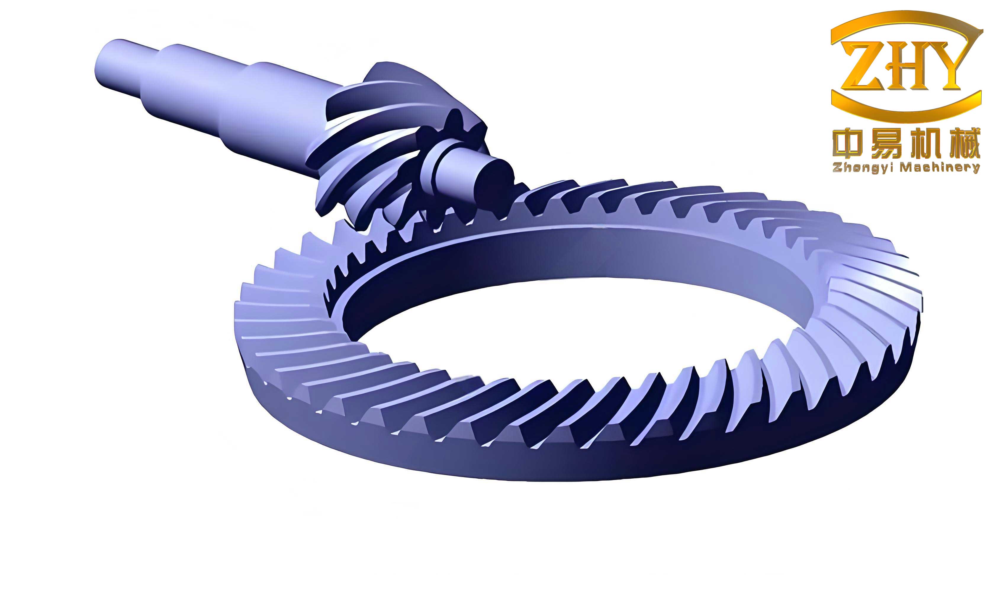
Contrary to any lingering perception of mystery, hyperbolic gears are highly refined mechanical components produced in the millions annually. Their successful, global application in vehicle drivetrains is a testament to their capability. The comprehensive geometric and kinematic foundation for hyperbolic gears was established in seminal works. This narrative aims to provide a clear, logical explanation of the geometry and kinematics, clarifying the meaning and interrelationships of terms encountered in the design and calculation of hyperbolic gears.
Geometry of Hyperbolic Gears: A Systematic Derivation
The design begins in three-dimensional space with two axes, typically non-intersecting, non-parallel, and non-perpendicular. A unique line, the common perpendicular or centerline, can be defined between these two axes. The distance measured along this line is the offset or hypoid distance, denoted as $E$. Let us designate one axis as the gear (or ring gear) axis and the other as the pinion axis. The angle between the axes, measured in a plane parallel to both, is the shaft angle, $\Sigma$. A crucial step is selecting the mean point $M$ where gear mesh action is intended to be centered. This point is defined by three parameters relative to the gear axis: its mean radius $r_{m2}$, its axial offset $z_m$, and its angular location $\theta_m$ in the gear’s plane of rotation.
Through point $M$, a line can be drawn intersecting both axes. This is the pitch normal. When viewed along the gear axis, its inclination is the angle $\alpha$; when viewed along the pinion axis, its inclination is the angle $\beta$. The distance from $M$ to the pinion axis is the pinion mean radius, $r_{m1}$. For simplicity, and common in automotive applications, we often assume the axes are perpendicular ($\Sigma = 90^\circ$), though the principles are general. From this spatial geometry, we can derive the formulas for the newly defined angles:
$$ \tan \alpha = \frac{E – z_m}{r_{m2}} $$
$$ \tan \beta = \frac{z_m}{r_{m1}} $$
A plane passed through point $M$ and perpendicular to the pitch normal is called the pitch plane. This plane intersects the gear axis at point $O_2$ (the gear pitch cone apex) and the pinion axis at point $O_1$ (the pinion pitch cone apex). The distance $O_2M$ is the gear pitch cone distance, $R_{m2}$, and $O_1M$ is the pinion pitch cone distance, $R_{m1}$. The angles between the axes and the pitch plane are the pitch cone angles: $\gamma_2$ for the gear and $\gamma_1$ for the pinion. Other key angles within the pitch plane are the supplemental shaft angle $\delta = 180^\circ – \Sigma$ and the angle between the cone generators, $\phi$. Simple and sufficient relationships can be written as:
$$ \sin \gamma_2 = \frac{r_{m2}}{R_{m2}} $$
$$ \sin \gamma_1 = \frac{r_{m1}}{R_{m1}} $$
$$ \cos \phi = \sin \gamma_1 \sin \gamma_2 \cos \delta + \cos \gamma_1 \cos \gamma_2 $$
Since the pitch normal intersects both axes and the pitch plane is perpendicular to it, a pair of cones tangent at $M$ can be conceptualized around each axis. The gear cone has its apex at $O_2$, and the pinion cone at $O_1$. The lengths of the cone elements to $M$ are the pitch cone distances $R_{m2}$ and $R_{m1}$. It is vital to understand that these “pitch cones” differ from those in parallel or intersecting axis gears. They do not roll without sliding; they are geometric constructs that serve as the basis for the blank design.
Determining Spiral Angle from Gear Ratio
The pitch plane view is critical for understanding velocity. Vector $\vec{\omega_2}$ is the gear angular velocity, and $\vec{\omega_1}$ is the pinion angular velocity. The position vector from the gear apex to point $M$ is $\vec{R_2}$, and from the pinion apex to $M$ is $\vec{R_1}$. The velocity of point $M$ as part of the gear is $\vec{V_2} = \vec{\omega_2} \times \vec{R_2}$, and as part of the pinion is $\vec{V_1} = \vec{\omega_1} \times \vec{R_1}$. The relative velocity vector at $M$ is:
$$ \vec{V_{12}} = \vec{V_1} – \vec{V_2} = \vec{\omega_1} \times \vec{R_1} – \vec{\omega_2} \times \vec{R_2} $$
This vector $\vec{V_{12}}$ lies in the pitch plane and determines the direction of the tooth trace. For contact at $M$ with a prescribed gear ratio, the fundamental law of gearing requires that the relative velocity has no component normal to the tooth surface: $\vec{V_{12}} \cdot \vec{n} = 0$, where $\vec{n}$ is the unit normal vector at the contact point.
The gear spiral angle $\psi_2$ is the angle between the tooth trace and the gear pitch cone element, and the pinion spiral angle $\psi_1$ is the corresponding angle on the pinion. The sliding velocity magnitude is $|\vec{V_{12}}|$. The spiral angles are fundamentally tied to the chosen mean point and the gear ratio $i = \omega_2 / \omega_1$. Well-known algebraic formulas are:
$$ \sin \psi_1 = \frac{r_{m2} + i r_{m1} \cos \Sigma}{i R_{m1}} $$
$$ \sin \psi_2 = \frac{i r_{m1} + r_{m2} \cos \Sigma}{R_{m2}} $$
The pressure angle can be chosen freely in a direction perpendicular to the tooth trace. However, if the resulting spiral angle is unsatisfactory, one of the parameters defining $M$ (typically $z_m$) must be adjusted.
| Symbol | Term | Governing Relationship |
|---|---|---|
| $E$ | Offset (Hypoid Distance) | Given design parameter |
| $\Sigma$ | Shaft Angle | Given design parameter (often $90^\circ$) |
| $r_{m2}$, $z_m$, $\theta_m$ | Gear Mean Point Coordinates | Primary design choices |
| $\alpha$, $\beta$ | Pitch Normal Angles | $\tan \alpha = (E – z_m)/r_{m2}$, $\tan \beta = z_m/r_{m1}$ |
| $\gamma_2$, $\gamma_1$ | Pitch Cone Angles | $\sin \gamma_2 = r_{m2}/R_{m2}$, $\sin \gamma_1 = r_{m1}/R_{m1}$ |
| $\psi_2$, $\psi_1$ | Spiral Angles | $\sin \psi_2 = (i r_{m1} + r_{m2} \cos \Sigma)/R_{m2}$ |
| $i$ | Gear Ratio | $i = \omega_2 / \omega_1$ |
Tooth Surfaces and the Concept of Limit Parameters
For a conjugate pair of hyperbolic gears, one can theoretically choose an arbitrary tooth profile for one member and derive the mating surface. The requirement $\vec{V_{12}} \cdot \vec{n} = 0$ forces the tooth direction as calculated. The characteristics of the chosen profile are studied via its path of contact. For optimal performance, two conditions are desired: both sides of the path of contact should be symmetrically inclined relative to the pitch plane, and they should intersect along a line tangent to the pitch plane. The first aims for equal overlap ratio and undercut avoidance on both flanks; the second prevents one end of the tooth from becoming pointed while the other is undercut.
The offset creates asymmetry, causing the inclination of the path of contact to differ from the nominal pressure angle. This leads to the concept of a special limit pressure angle, $\alpha_0$. A tooth surface with this pressure angle, generated as a surface of revolution about an axis perpendicular to the pitch plane, produces a path of contact exactly tangent to the pitch plane. It represents the “zero” pressure angle condition in hypoid geometry. Its value is derived from kinematic conditions and is given by:
$$ \tan \alpha_0 = \frac{\sin \psi_1 \sin \psi_2}{\sin(\psi_1 + \psi_2)} $$
Furthermore, this specific surface has a characteristic limit radius of curvature, $\rho_0$. When a cutter with this radius is used with the limit pressure angle, it generates the aforementioned tangent contact path. This radius serves as an excellent starting point for selecting the practical cutter radius. Its formula is:
$$ \rho_0 = R_{m1} \cdot \frac{\sin^2 \psi_2}{\sin \alpha_0 \sin(\psi_1 + \psi_2)} $$
Adjusting the initial design parameter $\theta_m$ allows the designer to tailor $\rho_0$ to match standard cutter sizes, just as adjusting $z_m$ tailors the spiral angle. Calculations for a typical automotive hyperbolic gear set using these limit parameters confirm that the paths of contact are only slightly curved and very close to the pitch plane, validating their use as fundamental design parameters.
| Parameter | Formula |
|---|---|
| Gear Spiral Angle, $\psi_2$ | $\sin \psi_2 = \dfrac{i r_{m1} + r_{m2} \cos \Sigma}{R_{m2}}$ |
| Pinion Spiral Angle, $\psi_1$ | $\sin \psi_1 = \dfrac{r_{m2} + i r_{m1} \cos \Sigma}{i R_{m1}}$ |
| Limit Pressure Angle, $\alpha_0$ | $\tan \alpha_0 = \dfrac{\sin \psi_1 \sin \psi_2}{\sin(\psi_1 + \psi_2)}$ |
| Limit Radius of Curvature, $\rho_0$ | $\rho_0 = R_{m1} \cdot \dfrac{\sin^2 \psi_2}{\sin \alpha_0 \sin(\psi_1 + \psi_2)}$ |
Crowned Teeth and the Nature of Tooth Contact
Theoretically conjugate hyperbolic gears are impractical as they are highly sensitive to manufacturing errors and assembly misalignments. To introduce necessary insensitivity and tolerance, the tooth surfaces are deliberately modified with a carefully chosen “crown.” This crowning, applied in both the lengthwise and profile directions, transforms the theoretical line contact into a point contact under no-load conditions. The size and shape of this crown directly determine the gear set’s ability to accommodate misalignment while maintaining smooth operation.
The quality of this crown is judged by the tooth contact pattern observed under light load on a testing machine. A well-designed crown produces a contact pattern centered on the tooth face and flank under nominal assembly conditions. The pattern’s behavior when the pinion position is intentionally misaligned reveals the crowning’s characteristics. Two classic adjustments are the change in axial pinion position ($\Delta P$) and the change in offset ($\Delta E$). The ratio $\Delta E / \Delta P$ required to move the contact pattern from the toe to the heel of the tooth while keeping it at a constant height is a key indicator, often called the “$E/P$ test value.” Diagonal contact patterns can also be engineered for specific smoothness requirements.
While visual inspection and acoustic judgment are traditional, a quantitative analytical method called Tooth Contact Analysis (TCA) has been developed. TCA mathematically simulates the meshing of crowned hyperbolic gears at any specified relative position, calculating the contact point path, transmission errors, and the size/orientation of the instantaneous contact ellipse. This provides a theoretical prediction of the contact pattern and the $E/P$ value without physical prototypes.
The mathematical core of TCA is an iterative numerical procedure. It starts with arbitrary candidate points on both tooth surfaces, defined by their manufacturing parameters (e.g., cradle angle $\theta_c$ and cutter rotation $\phi$ for a generated tooth). The algorithm virtually moves the gears until these points and their surface normals coincide, establishing a potential contact point. It then iteratively adjusts the candidate parameters until the actual operating position (specified offset $E$, shaft angle $\Sigma$, and axial positions) is satisfied. For each converged contact point, TCA computes the local surface curvatures, which define the contact ellipse, and the kinematic motion transfer. Repeating this for various roll positions maps the entire contact path and predicts the no-load contact pattern.
Strength Calculation for Hyperbolic Gears
The final pillar of hyperbolic gear design is ensuring sufficient strength under load. The ideal contact pattern under load is a broad, uniform area across the tooth face. Achieving this in practice requires coordination between design, manufacturing, and assembly, considering constraints of weight, cost, and space. Bearing arrangement is critical; a straddle-mounted design generally imposes lower loads on bearings than an overhung (cantilever) design, allowing for smaller, lighter components for equivalent stiffness. However, spatial constraints often dictate the final layout.
Strength calculations for hyperbolic gears follow principles similar to other gear types but account for their unique geometry and high sliding components. Two primary failure modes are addressed: bending fatigue at the tooth root and surface durability (pitting) on the flanks.
Bending Strength: The Lewis formula provides the foundational concept, modified with a comprehensive set of application factors. The bending stress $\sigma_b$ is calculated as:
$$ \sigma_b = \frac{F_t}{b m_n} \cdot \frac{1}{Y} \cdot K_A \cdot K_V \cdot K_{H\beta} \cdot K_{F\alpha} $$
Where $F_t$ is the tangential force at the mean cone distance, $b$ is the face width, $m_n$ is the normal module, $Y$ is the tooth form factor (dependent on number of teeth, pressure angle, and addendum), and the $K$ factors account for application ($K_A$), dynamic load ($K_V$), load distribution across the face width ($K_{H\beta}$), and load sharing between simultaneous tooth pairs ($K_{F\alpha}$). For hyperbolic gears, the force calculation must correctly resolve the three-dimensional force components due to the shaft offset and spiral angles.
Surface Durability (Pitting Resistance): The contact stress $\sigma_H$ is governed by the Hertzian theory for contacting cylinders, adapted for gear teeth. The fundamental formula is:
$$ \sigma_H = Z_E \sqrt{ \frac{F_t}{b d_{m1}} \cdot \frac{u+1}{u} \cdot K_A \cdot K_V \cdot K_{H\beta} \cdot K_{H\alpha} } $$
Here, $Z_E$ is the elasticity factor $\sqrt{ \frac{1}{\pi ( \frac{1-\nu_1^2}{E_1} + \frac{1-\nu_2^2}{E_2} ) } }$, $d_{m1}$ is the pinion mean diameter, $u$ is the gear ratio ($z_2/z_1$), and $K_{H\alpha}$ is the transverse load factor. For hyperbolic gears, additional considerations include the high sliding velocities, which influence lubrication regime and heat generation, and the need for extreme pressure (EP) additives in the lubricant to prevent scuffing. The effective radii of curvature at the contact point, derived from the TCA geometry, are crucial inputs for an accurate contact stress calculation.
| Failure Mode | Governing Stress Formula | Key Influencing Factors for Hypoid Gears |
|---|---|---|
| Bending Fatigue | $\sigma_b = \dfrac{F_t}{b m_n Y} \cdot K_A \cdot K_V \cdot K_{H\beta} \cdot K_{F\alpha}$ | 3D force resolution, localized stress due to crowning, spiral angle effect on form factor $Y$. |
| Surface Pitting | $\sigma_H = Z_E \sqrt{ \dfrac{F_t}{b d_{m1}} \cdot \dfrac{u+1}{u} \cdot K_A \cdot K_V \cdot K_{H\beta} \cdot K_{H\alpha} }$ | Hertzian contact with curvatures from TCA, high sliding velocities, lubricant EP additives, thermal effects. |
In conclusion, the engineering of hyperbolic gears is a sophisticated synthesis of spatial geometry, kinematic analysis, controlled surface modification, and rigorous strength verification. From the initial layout of offset axes and the mean point selection, through the determination of spiral angles and limit geometry, to the precise crowning defined via TCA and the final validation against bending and contact stress limits, each step is interconnected. The successful application of millions of hyperbolic gears in demanding automotive environments stands as proof that this complex system of design and analysis is both well-understood and highly effective. The continuous refinement of methods like TCA ensures that the performance and reliability of these vital components will only improve.