
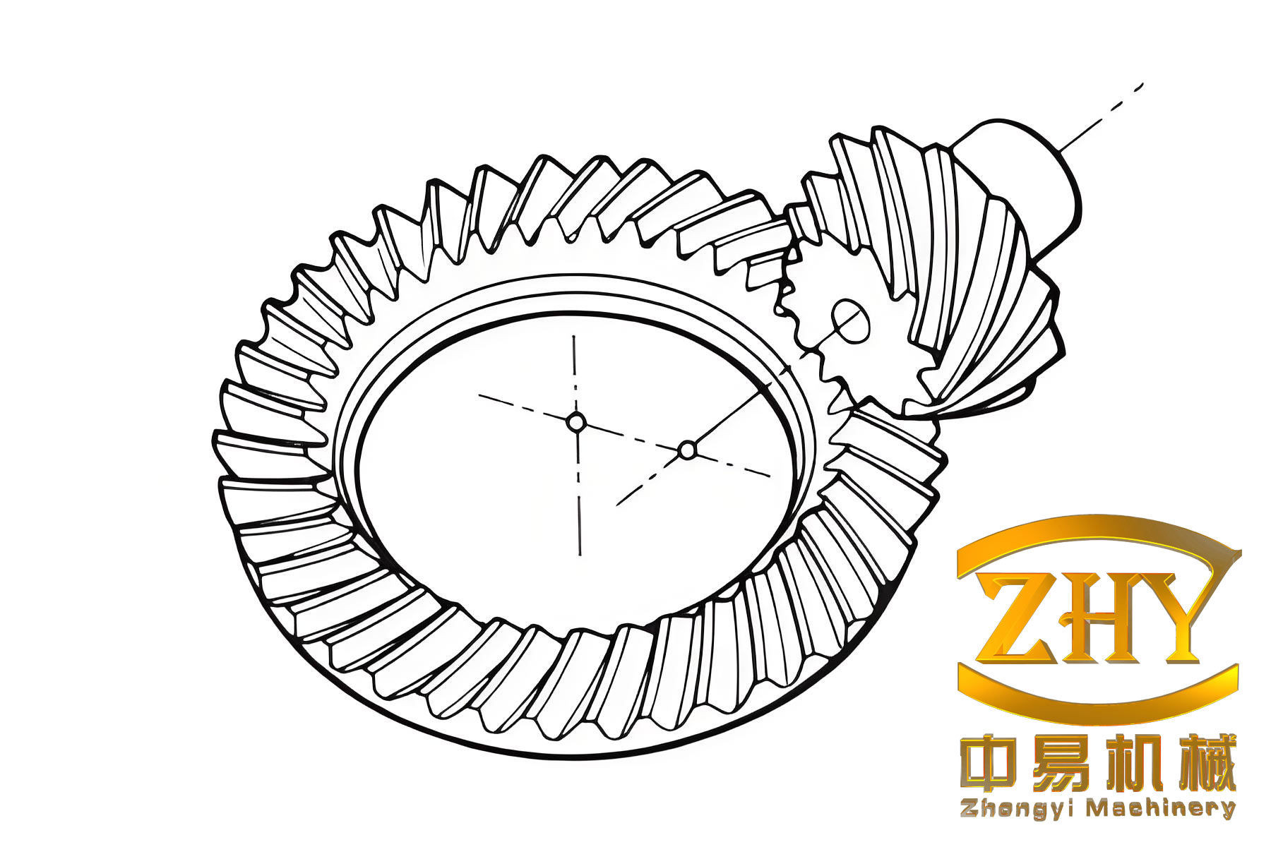
In the realm of automotive powertrain systems, the final drive axle plays a critical role in transmitting torque from the propeller shaft to the driving wheels while providing the necessary speed reduction and torque multiplication. At the heart of this assembly lies the main reducer, a component whose performance and reliability are paramount for vehicle dynamics, fuel efficiency, and NVH (Noise, Vibration, and Harshness) characteristics. Among the various gear geometries employed for this task, the hypoid bevel gear has become the predominant choice for modern automotive applications. Its defining feature is the offset between the axes of the pinion and the ring gear, which allows for a lower overall vehicle profile and more flexible drivetrain packaging. Furthermore, the hypoid bevel gear mesh is characterized by a combination of rolling and longitudinal sliding motion, coupled with a high pinion spiral angle. This results in a larger average number of teeth in contact during operation compared to straight or spiral bevel gears, leading to smoother power transmission, higher load-carrying capacity, and significantly lower operational noise.
However, the superior performance of the hypoid bevel gear comes at the cost of heightened sensitivity to manufacturing inaccuracies and assembly errors. The complex tooth geometry and the high degree of conformity in the mesh mean that even minor deviations from the ideal design can lead to premature failure, increased vibration, and unacceptable noise levels. Traditional quality assessment methods in production, such as visual inspection of gear contact patterns (ink testing) or subjective auditory evaluation for “abnormal noises,” are heavily reliant on operator skill and are inherently qualitative and inconsistent. These methods fail to provide the quantitative, objective, and repeatable data required for modern statistical process control and predictive maintenance. Consequently, there is a compelling need for an advanced, signal-based diagnostic methodology that can reliably assess the health state of a hypoid bevel gear reducer directly on the assembly line, such as during its run-in or testing cycle.
This article presents a comprehensive fault diagnosis framework for hypoid bevel gear main reducers, leveraging vibration analysis as the primary sensing modality. The core premise is that the dynamic forces generated by gear meshing, and more importantly, by any faults within the system, are directly transmitted to the gearbox housing where they can be measured as vibration signals. By applying advanced signal processing techniques to extract meaningful features and employing artificial intelligence for pattern recognition, we can move from mere anomaly detection to precise fault identification and quality grading.
Typical Failure Modes in Hypoid Bevel Gear Manufacturing
The journey of a hypoid bevel gear from raw forging to a finished component in an axle is fraught with potential sources of quality degradation. Understanding these failure modes is essential for designing an effective diagnostic system.
1. Heat Treatment Distortion: This is arguably the most significant and challenging issue. The carburizing and quenching process, necessary for achieving a hard, wear-resistant case and a tough core, induces complex thermal and phase transformation stresses. Distortion manifests as changes in gear geometry – lead angle deviation, profile error, and helix distortion – which directly degrade the quality of meshing. Studies suggest the influence is partitioned approximately as follows: 50-60% due to part design and geometry, 20-30% due to material properties (hardenability, homogeneity), and 5-15% due to the specifics of the heat treatment process itself (furnace atmosphere, quenching medium, fixturing).
| Factor Category | Key Elements | Influence on Distortion |
|---|---|---|
| Design & Geometry | Module, wall thickness, symmetry, shape complexity | Highest influence. Simple, symmetric, uniform sections distort less. |
| Material Properties | Hardenability, chemical homogeneity, purity | Medium-high influence. Non-uniformity leads to uneven stresses and distortion. |
| Heat Treatment Process | Carburizing parameters, quenching rate & uniformity, tempering temperature | Medium influence. Unstable cooling promotes unwanted microstructures (e.g., bainite) affecting final dimensions. |
The material’s hardenability is particularly critical. Excessive hardenability can increase warpage and risk of quenching cracks, while insufficient hardenability leads to low core hardness, predisposing the gear to bending fatigue and deep spalling failures.
2. Assembly and Installation Errors: Even a perfectly manufactured gear set can perform poorly if incorrectly assembled into the differential carrier. Key installation parameters include:
– Pinion Mounting Distance: The axial position of the pinion relative to the gear center.
– Gear Backlash: The clearance between mating tooth flanks.
– Pinion Offset Setting: Maintaining the designed hypoid offset.
Deviations in these settings alter the contact pattern, shifting it towards the toe, heel, or edges of the tooth, leading to localized stress concentrations, rapid wear, and noise.
3. Surface Defects: These include nicks, dents, or burrs incurred during handling, as well as more subtle manufacturing defects like grinding burns or soft spots due to improper carburizing. A common, severe defect is a “hard spot” or “inclusion” (sometimes referred to as a “包块” or lump in the material structure), which creates a pronounced, periodic impact every time it enters the mesh.
All these faults modulate the normal vibration signature of the gearbox. Our diagnostic approach aims to detect and classify these modulations.
Methodology: From Vibration to Diagnosis
Theoretical Basis: Vibration as a Proxy for Acoustic Emission
The choice of vibration analysis is grounded in fundamental acoustics. In a mechanical system, vibration is the source of structure-borne noise. The sound power radiated from a vibrating surface is directly proportional to its mean-square vibration velocity. A simplified relationship can be expressed as:
$$W = \rho c S \sigma_r \bar{V^2}$$
where:
– $W$ is the radiated sound power.
– $\rho$ is the density of the medium (air).
– $c$ is the speed of sound.
– $S$ is the radiating surface area.
– $\sigma_r$ is the radiation efficiency.
– $\bar{V^2}$ is the spatially and temporally averaged mean-square vibration velocity.
This principle validates the use of vibration monitoring for quality assessment traditionally done by noise evaluation. Any fault that increases gear mesh excitation will increase the vibration response of the housing, which in turn increases the radiated noise. Vibration signals offer practical advantages: they are easier to measure reliably in noisy industrial environments using accelerometers, they provide a direct measure of the structural dynamics, and a rich body of signal processing techniques exists for their analysis.
Signal Processing and Feature Extraction Pipeline
The raw vibration signal from a run-in test is non-stationary and contains information across a broad frequency band. The diagnostic pipeline involves processing this signal to extract a compact set of numerical descriptors, or “features,” that are sensitive to different fault conditions but insensitive to normal operational variations.
1. Time-Domain Statistical Features:
These features are calculated directly from the discrete-time vibration signal $x[n]$ of length $N$. They can be divided into dimensional and dimensionless parameters. Dimensional parameters (e.g., RMS) are sensitive to overall energy levels but can be affected by load and speed. Dimensionless parameters (e.g., kurtosis) describe the shape of the signal distribution and are often more robust indicators of fault-induced impulsivity.
| Feature | Formula | Sensitivity to Hard Spot/Lump | Sensitivity to General Noise/Incorrect Mesh |
|---|---|---|---|
| Root Mean Square (RMS) | $X_{rms} = \sqrt{\frac{1}{N}\sum_{i=1}^{N} x[i]^2}$ | High | High |
| Variance | $\sigma^2 = \frac{1}{N}\sum_{i=1}^{N} (x[i] – \mu_x)^2$ | High | High |
| Kurtosis | $\beta = \frac{1}{N}\sum_{i=1}^{N} x[i]^4$ | Very High (excellent for impacts) | Low |
| Kurtosis Indicator | $K = \beta / X_{rms}^4$ | Very High | Moderate |
| Clearance Indicator (L) | $L = \frac{\max(|x[i]|)}{(\frac{1}{N}\sum \sqrt{|x[i]|})^2}$ | High | Moderate |
| 6th & 8th Order Normalized Moments | $R_6 = \frac{\sum x[i]^6}{N\sigma^6}$, $R_8 = \frac{\sum x[i]^8}{N\sigma^8}$ | Very High | Low |
Kurtosis and higher-order moments are exceptionally sensitive to the transient impacts caused by a localized defect like a hard spot on a hypoid bevel gear tooth.
2. Frequency-Domain Features:
The Power Spectral Density (PSD), $P(f)$, represents the signal’s energy distribution across frequency. Faults often alter this distribution.
- Spectral Centroid (FC): Indicates the “center of mass” of the spectrum. A shift can imply changing frequency content.
$$FC = \frac{\sum_{i=1}^{M} f_i P(f_i)}{\sum_{i=1}^{M} P(f_i)}$$ - Spectral Variance (VF): Measures the spread of the spectrum. A fault may concentrate or disperse energy.
$$VF = \frac{\sum_{i=1}^{M} (f_i – FC)^2 P(f_i)}{\sum_{i=1}^{M} P(f_i)}$$ - Mean Square Frequency (MSF): A measure related to the average frequency component weighted by power.
$$MSF = \frac{\sum_{i=1}^{M} f_i^2 P(f_i)}{\sum_{i=1}^{M} P(f_i)}$$
3. Time-Frequency Analysis via Wavelet Packet Decomposition (WPD):
Fourier analysis assumes stationarity and loses temporal information. The Short-Time Fourier Transform (STFT) has a fixed resolution window. For the non-stationary, transient-rich signals from faulty hypoid bevel gears, Wavelet Packet Decomposition is superior. It generalizes the wavelet transform by iteratively decomposing both the low-frequency and high-frequency subbands, creating a complete binary tree. At depth $d$, the signal is decomposed into $2^d$ frequency subbands of equal bandwidth, providing a fine-grained, adaptive time-frequency representation. The energy of the coefficients in each subband $E_j$ is computed as a potent feature:
$$E_j = \sum_{k} |C_{j,k}|^2$$
where $C_{j,k}$ are the wavelet packet coefficients for node $j$. For a hypoid bevel gear signal, certain subbands will contain more energy related to mesh harmonics, sidebands, or fault-induced resonances. Daubechies wavelets (e.g., ‘db4’, ‘db8’) are commonly used for their orthogonality and good locality properties.
Intelligent Fault Classification with BP Neural Networks
The extracted feature vector (e.g., combining 6 time-domain stats and 6 WPD subband energies) forms the input to a pattern classifier. The Backpropagation (BP) Neural Network is a workhorse for this task due to its universal approximation capability and ability to learn complex, non-linear mappings between features and fault classes.
Network Architecture & Design:
A typical three-layer feedforward network is sufficient: an Input Layer, one Hidden Layer, and an Output Layer.
- Input Layer: Number of neurons equals the dimension of the feature vector (e.g., 12).
- Hidden Layer: The number of neurons is determined empirically. A starting point can be $\sqrt{n_{input} \cdot n_{output}} + \alpha$, where $\alpha$ is a small integer (e.g., 2-5). For 12 inputs and 3 outputs, 7-10 neurons is a reasonable range to test.
- Output Layer: Number of neurons equals the number of fault classes. For a 3-class problem (Normal, Hard Spot, Poor Mesh/Noise), we use three neurons. The target output is encoded as: Normal = [1,0,0]; Hard Spot = [0,1,0]; Poor Mesh = [0,0,1].
The mathematical model for a neuron’s output is:
$$y_j = f\left(\sum_{i=1}^{n} w_{ij} x_i + b_j\right)$$
where $f(\cdot)$ is the activation function, $w_{ij}$ are the connection weights, $x_i$ are inputs, and $b_j$ is the bias. Common choices are the hyperbolic tangent (`tansig`) for hidden layers and the logistic sigmoid (`logsig`) for the output layer for classification.
Training and Generalization:
The network is trained using a set of labeled feature vectors from known good and faulty hypoid bevel gear reducers. The Scaled Conjugate Gradient (SCG) algorithm is often preferred over standard gradient descent for its faster convergence. To prevent overfitting and improve generalization to new, unseen data, techniques like early stopping (using a separate validation set) and regularization (adding a penalty term for large weights to the error function) are employed. The error function during training is often a regularized mean squared error:
$$E_{reg} = \gamma \cdot \text{MSE} + (1-\gamma) \cdot \text{MSW}$$
where $\text{MSE}$ is the mean square error, $\text{MSW}$ is the mean square of the network weights, and $\gamma$ is the performance ratio parameter.
| Network Component | Configuration / Choice | Rationale |
|---|---|---|
| Input Vector | 12 dimensions: Variance, RMS, Kurtosis Ind., Clearance Ind., R6, R8, and energies from 6 selected WPD nodes. | Combines sensitivity to impulsivity (time stats) and specific frequency band energy (WPD). |
| Hidden Layer | 9 neurons (determined experimentally). | Provides sufficient complexity to model fault patterns without overfitting. |
| Output Layer | 3 neurons (Normal, Hard Spot, Poor Mesh). | Encodes the three primary quality states. |
| Hidden Activation | `tansig` (Hyperbolic tangent sigmoid) | Provides non-linearity and outputs in range [-1,1]. |
| Output Activation | `logsig` (Logistic sigmoid) | Squashes output to [0,1], interpretable as probability. |
| Training Algorithm | Scaled Conjugate Gradient (SCG) | Faster convergence for pattern recognition problems. |
| Regularization | Performance Ratio (γ) set to 0.7-0.9 | Penalizes large weights to improve network generalization. |
Implementation and Validation Case Study
The proposed system was implemented in a hybrid programming environment. Data acquisition from an IEPE accelerometer mounted on the differential housing during the run-in test was managed via a National Instruments data acquisition card and controlled by a LabVIEW virtual instrument (VI). The core signal processing and classification algorithms, including WPD and the BP neural network, were developed in MATLAB for their robust numerical and AI toolboxes. The MATLAB scripts were seamlessly integrated into the LabVIEW VI using the `MATLAB Script Node`, creating a cohesive, automated testing station.
Procedure:
1. Data Collection: Vibration signals were collected from a batch of hypoid bevel gear reducers, including units confirmed as normal, units with induced hard spot defects, and units with assembly errors causing poor meshing and noise.
2. Training Phase: For each unit, the 12-dimensional feature vector was computed. A set of 18 feature vectors (6 from each class) was used to train the BP network. The network’s weights and biases were iteratively adjusted to minimize the error between its predicted output and the known target class vectors.
3. Testing/Validation Phase: The trained network was then presented with feature vectors from a separate, unseen set of 9 reducers (3 from each class). The network’s output for each test sample is a 3-element vector, where each element can be interpreted as the network’s “confidence” or probability that the sample belongs to the corresponding class.
Results and Interpretation:
The network’s performance on the test set was exemplary. For nearly all test samples, the network assigned a probability greater than 99% to the correct fault class. The table below shows a subset of the results. For instance, a normal gearbox yielded an output vector of [0.9994, 0.0050, 0.0079], strongly indicating the “Normal” class. A hard spot fault produced [0.0062, 0.9942, 0.0070], and a poor mesh unit resulted in [0.0002, 0.0044, 0.9999].
| Unit Type (Ground Truth) | Ideal Target Output | Actual Network Output [Norm, Spot, Noise] | Implied Classification |
|---|---|---|---|
| Normal Unit #1 | [1, 0, 0] | [0.9994, 0.0050, 0.0079] | Normal (99.94% confidence) |
| Normal Unit #2 | [1, 0, 0] | [0.9999, 0.0020, 0.0005] | Normal (99.99% confidence) |
| Hard Spot Unit #1 | [0, 1, 0] | [0.0062, 0.9942, 0.0070] | Hard Spot (99.42% confidence) |
| Hard Spot Unit #2 | [0, 1, 0] | [0.2988, 0.9258, 0.0070] | Hard Spot (92.58% confidence)* |
| Poor Mesh Unit #1 | [0, 0, 1] | [0.0002, 0.0044, 0.9999] | Poor Mesh (99.99% confidence) |
| Poor Mesh Unit #3 | [0, 0, 1] | [0.0367, 0.0000, 0.8540] | Poor Mesh (85.40% confidence) |
* Note: Unit #2 with a hard spot showed some characteristic of a normal unit (29.88% probability), suggesting a possibly less severe defect or the presence of mixed conditions, yet the diagnosis remains correct and more nuanced than a simple pass/fail.
This demonstrates the system’s capability not only for binary pass/fail judgment but also for multi-class fault identification, providing specific feedback (e.g., “hard spot detected” vs. “general meshing issue”) that is invaluable for root cause analysis and process correction in the manufacturing of hypoid bevel gear sets.
Conclusion
This article has detailed an advanced, intelligent framework for the fault diagnosis and quality assessment of automotive hypoid bevel gear main reducers. By moving away from subjective manual inspections and embracing data-driven vibration analysis, the method achieves a high degree of objectivity, repeatability, and precision. The synergy of signal processing techniques—using both traditional time/frequency statistics and modern wavelet packet decomposition—enables the extraction of a rich, discriminative feature set that captures the unique signatures of different fault modes. The subsequent use of a trained Backpropagation neural network provides a powerful, adaptive tool for automatically classifying the condition of a gear set based on these features.
The implemented system, built on a LabVIEW-MATLAB hybrid platform, proves effective in distinguishing between normal units, those with localized material defects (hard spots), and those suffering from assembly-related poor meshing. The high classification accuracy on validation data underscores the practical viability of this approach for integration into end-of-line testing stations. It offers manufacturers a significant upgrade in quality control for hypoid bevel gear production, enabling faster feedback, reduced reliance on skilled labor, and ultimately, the delivery of more reliable and quieter automotive drivetrains. Future work may explore deep learning architectures like Convolutional Neural Networks (CNNs) operating directly on time-frequency images (scalograms) or the incorporation of additional sensor data (e.g., acoustic emission, torque) for an even more comprehensive health monitoring system.