
In the realm of gear transmission systems, hypoid bevel gears play a pivotal role due to their ability to transmit motion between non-intersecting axes with high efficiency and smooth operation. These gears are extensively used in automotive differentials, aerospace applications, and heavy machinery, where precise meshing and durability are critical. However, the complex geometry of hypoid bevel gears, especially the fillet or transition surfaces between the tooth flank and root, poses significant challenges for accurate three-dimensional geometric modeling. Traditional modeling approaches often simplify these surfaces, leading to inaccuracies in subsequent analyses such as finite element analysis (FEA), dynamic contact analysis, and load distribution studies. This article presents a comprehensive method for deriving exact mathematical models of hypoid bevel gear tooth surfaces, including fillets, based on the HFT (Hypoid Gear Formate Tilt) machining process. By integrating kinematic principles of traditional cradle-type machines with virtual manufacturing simulations in CATIA, we establish a robust framework for generating precise 3D geometric models. The methodology not only ensures high fidelity in representing hypoid bevel gear geometry but also facilitates advanced engineering simulations, ultimately enhancing design optimization and performance prediction in real-world applications.
The HFT machining method is widely employed for manufacturing hypoid bevel gears, as it incorporates additional degrees of freedom such as tool tilt and rotation to achieve desired tooth modifications and localized contact patterns. In this process, a hypothetical crown gear, concentric with the machine cradle, engages with the workpiece through a series of coordinated motions. The cutting tool, typically a face-mill cutter with defined blade geometry, replicates the tooth surface of this crown gear, gradually generating the gear teeth on the blank via an enveloping process. Understanding the kinematic relationships between machine components—such as the cradle, tool head, eccentric cam, and workpiece—is essential for deriving accurate tooth surface equations. This involves establishing multiple coordinate systems and employing homogeneous coordinate transformations to describe relative positions and velocities during cutting. The complexity arises from the tool’s fillet region, where the blade edge transitions smoothly from the side-cutting edge to the top edge, necessitating precise mathematical representation to avoid stress concentrations and ensure gear strength.
To begin, we define the geometry of the cutting tool. The tool consists of side-cutting edges and a fillet region, typically modeled as a circular arc that tangentially connects the side and top edges. The parametric equations for the fillet region and side-cutting edge are expressed in the tool coordinate system. For the fillet region, let $\rho_f$ be the fillet radius, $\alpha_p$ the tool pressure angle, $R_p$ the cutter point radius, and $\lambda_f$ an angular parameter. The position vector and normal vector for a point on the fillet are given by:
$$r_p^{(b)}(\lambda_f, \theta) = \begin{bmatrix} (X_f – \rho_f \sin(\lambda_f)) \cos \theta \\ (X_f – \rho_f \sin(\lambda_f)) \sin \theta \\ -\rho_f (1 – \cos(\lambda_f)) \end{bmatrix}, \quad n_1 = \begin{bmatrix} \sin(\lambda_f) \cos \theta \\ \sin(\lambda_f) \sin \theta \\ \cos(\lambda_f) \end{bmatrix},$$
where $X_f = R_p \pm \rho_f \frac{1 – \sin(\alpha_p)}{\cos(\alpha_p)}$, with the sign depending on whether the convex or concave side is being cut. For the side-cutting edge, parameterized by $S_p$ (distance from the fillet) and $\theta$, we have:
$$r_p^{(a)}(S_p, \theta) = \begin{bmatrix} (R_p – S_p \sin \alpha_p) \cos \theta \\ (R_p – S_p \sin \alpha_p) \sin \theta \\ -S_p \cos \alpha_p \end{bmatrix}, \quad n_2 = \begin{bmatrix} \cos \alpha_p \cos \theta \\ \cos \alpha_p \sin \theta \\ \sin \alpha_p \end{bmatrix}.$$
These equations describe the tool surface geometry, which serves as the generating surface for the hypoid bevel gear tooth. The tool’s orientation and position are adjusted through tool tilt and rotation mechanisms, which are critical for achieving the desired tooth surface modifications in HFT machining.
The kinematic chain of a Gleason No. 116 cradle-type hypoid gear generator involves several coordinate transformations. We define coordinate systems attached to key machine components: the tool, tool tilt body, tool rotation body, eccentric cam, cradle, machine base, and workpiece. Using homogeneous transformation matrices, we relate these systems to derive the tool surface position in the workpiece coordinate system. Let $M_I$, $M_J$, $M_\beta$, and $M_Q$ represent transformation matrices for tool tilt angle $I$, tool rotation angle $J$, eccentric cam angle $\beta$, and cradle angle $Q$, respectively. The combined transformation from the tool coordinate system to the cradle coordinate system is:
$$M_{yd} = M_Q M_\beta M_J M_I.$$
Subsequently, considering the cradle rotation $q = \omega_1 t$ (where $\omega_1$ is the cradle angular velocity), bed slide motion $X_b$, workpiece installation angle $d$, and vertical offset $E_1$, we define transformations from the cradle to the workpiece. The transformation from the cradle coordinate system to the workpiece moving coordinate system is:
$$M_{Ld} = M_L M_x M_d M_q,$$
where $M_q$ accounts for cradle rotation, $M_d$ for workpiece installation, $M_x$ for horizontal offset $X_1$, and $M_L$ for workpiece rotation $\phi = i_{02} \omega_1 t$ with $i_{02}$ as the roll ratio. Thus, the tool surface point in the workpiece moving coordinate system is:
$$R_2 = M_{Ld} M_{yd} r_1,$$
where $r_1$ is the point vector in the tool coordinate system. This equation encapsulates the spatial relationship between the tool and workpiece during cutting, forming the basis for deriving the enveloping surface—the hypoid bevel gear tooth surface.
The generation of the tooth surface requires satisfying the meshing condition, which states that at the point of contact, the relative velocity between the tool and workpiece must be orthogonal to the common normal vector. The relative velocity vector $\mathbf{v}^{(12)}$ is derived from the kinematic chain:
$$\mathbf{v}^{(12)} = \boldsymbol{\omega}^{(12)} \times \mathbf{r}_1 + \frac{d\boldsymbol{\xi}}{dt} – \boldsymbol{\omega}_2 \times \boldsymbol{\xi},$$
where $\boldsymbol{\omega}^{(12)} = \boldsymbol{\omega}_1 – \boldsymbol{\omega}_2$, with $\boldsymbol{\omega}_1 = 0$ (tool rotation is negligible for surface generation) and $\boldsymbol{\omega}_2 = i_{02} \omega_1$ (workpiece rotation). The vector $\boldsymbol{\xi}$ represents the distance between coordinate origins, computed as:
$$\boldsymbol{\xi} = M_q M_{yd} \mathbf{E} – M_d^{-1} M_{Ld}^{-1} \mathbf{E}, \quad \mathbf{E} = [0, 0, 0, 1]^T.$$
The normal vector in the fixed coordinate system is $\mathbf{n} = M_q M_{yd} \mathbf{n}_1$. The meshing equation is then:
$$\mathbf{n} \cdot \mathbf{v}^{(12)} = F(\lambda_f, \theta, t) = 0.$$
Solving this equation yields a relation $\lambda_f = G(\theta, t)$, which, when substituted into $R_2$, provides the explicit tooth surface equation:
$$R_2 = \mathbf{g}(\theta, t).$$
This parametric form describes both the active tooth flank and the fillet region of the hypoid bevel gear, accounting for the entire cutting process. The complexity of these equations underscores the need for computational tools to handle the extensive algebraic expressions involved.
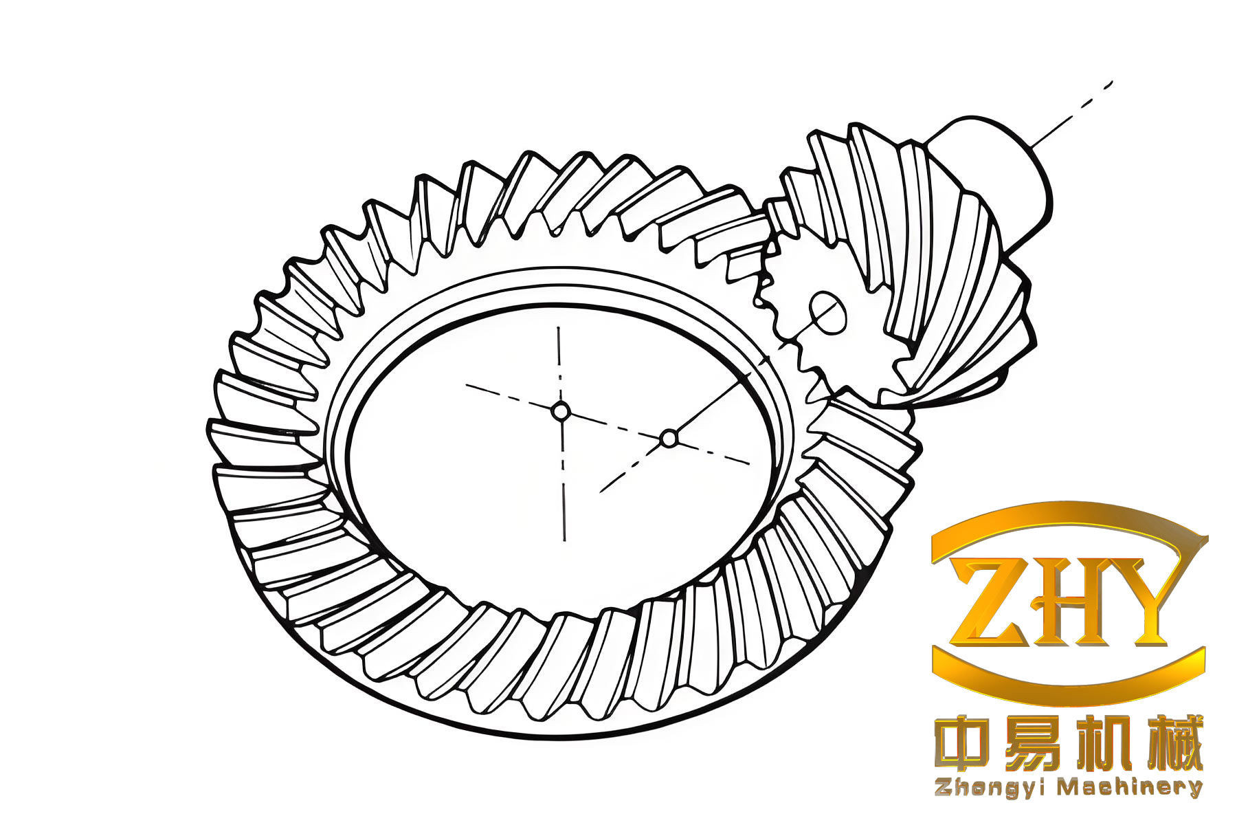
To facilitate practical application, we employ virtual manufacturing techniques using CATIA V5. This approach simulates the actual machining process by digitally replicating the machine kinematics and tool-workpiece interactions. The steps involve: (1) defining the machine environment with adjustable parameters (e.g., tool tilt, cradle angle), (2) positioning the tool and workpiece based on initial settings, (3) performing Boolean subtraction operations to simulate material removal at discrete time intervals, and (4) generating a family of enveloping curves that represent successive tool positions. These curves are then fitted using NURBS (Non-Uniform Rational B-Spline) surfaces to reconstruct a smooth, accurate 3D model of the hypoid bevel gear, including the fillet surfaces. The virtual process mirrors the mathematical derivation, providing a visual and geometric validation of the theoretical model. Below is an illustrative image depicting the setup for hypoid bevel gear machining in a virtual environment.
The accuracy of the virtual model is verified by comparing it with discrete points computed from the mathematical equations using MATLAB. For this purpose, we consider a specific hypoid bevel gear pair with parameters listed in Table 1. The gear data includes tooth numbers, diameters, angles, and dimensions essential for both mathematical computation and virtual modeling.
| Gear | Number of Teeth | Pitch Diameter (mm) | Outer Diameter (mm) | Pitch Cone Angle (°) | Face Cone Angle (°) | Root Cone Angle (°) | Circular Tooth Height (mm) | Normal Circular Thickness (mm) | Face Width (mm) |
|---|---|---|---|---|---|---|---|---|---|
| Pinion | 6 | 72.93 | 99.29 | 10.08 | 13.72 | 9.63 | 9.58 | 15.12 | 67.46 |
| Gear | 41 | 416.76 | 417.35 | 79.73 | 80.18 | 54.15 | 76.02 | 6.98 | 62.00 |
Additionally, the machine settings for finishing cuts on a Gleason No. 116 machine are provided in Table 2. These adjustments include tool positioning angles, offsets, and roll ratios, which directly influence the tooth surface geometry.
| Gear | Root Cone Angle (°) | Horizontal Offset (mm) | Bed Slide (mm) | Vertical Offset (mm) | Eccentric Cam Angle (°) | Cradle Angle (°) | Roll Ratio | Cutter Point Diameter (mm) | Tool Pressure Angle (°) | Fillet Radius (mm) |
|---|---|---|---|---|---|---|---|---|---|---|
| Pinion (Concave) | -2.00 | -7.98 | 17.08 | 29.12 | 81.90 | 112.20 | 6.33912 | 285.52 | 20 | 2.59 |
| Pinion (Convex) | -3.98 | 9.76 | 22.61 | 42.62 | 102.13 | 104.93 | 7.26721 | 328.94 | 25 | 2.59 |
| Gear | 76.40 | -1.10 | 100.09 | 122.43 | – | – | – | 304.80 | 22.50 | 2.29 |
Using MATLAB, we discretize the parameters $\theta$ and $t$ over specified ranges to compute points on the tooth surface from the derived equations. The algorithm involves solving the meshing equation numerically for each parameter pair, then evaluating $R_2$ to obtain coordinates. These discrete points are imported into CATIA and superimposed on the virtual model for error analysis. The normal deviations between the mathematical points and the virtual surface are measured at multiple locations across the tooth flank and fillet. Table 3 presents a subset of these error values, demonstrating the high precision achieved.
| Point Index | 1 | 2 | 3 | 4 | 5 | 6 | 7 | 8 | 9 |
|---|---|---|---|---|---|---|---|---|---|
| 1 | -0.1 | -0.062 | -0.097 | -0.930 | -0.009 | 0.096 | 0.074 | 0.058 | 0.065 |
| 2 | -0.087 | -0.074 | -0.085 | -0.075 | -0.007 | 0.093 | 0.042 | 0.045 | 0.050 |
| 3 | -0.080 | -0.085 | -0.074 | -0.020 | 0.000 | 0.091 | 0.013 | 0.056 | 0.044 |
| 4 | -0.078 | -0.097 | -0.062 | 0.038 | -0.004 | 0.089 | 0.094 | 0.037 | 0.039 |
| 5 | -0.081 | -0.099 | -0.051 | 0.099 | 0.010 | 0.085 | 0.083 | 0.028 | 0.038 |
The errors are within ±0.1 μm for most points, confirming the virtual model’s accuracy. This level of precision is sufficient for demanding engineering analyses, such as tooth contact pattern evaluation, stress distribution studies, and dynamic simulation of hypoid bevel gear pairs. The seamless integration of mathematical modeling and virtual manufacturing thus provides a reliable digital twin of the physical gear, enabling designers to optimize geometry before actual production.
Beyond the basic modeling, several enhancements can be incorporated to address specific design requirements. For instance, tooth surface modifications—such as crowning, bias, and spiral angle adjustments—are often applied to improve meshing performance and reduce noise. These modifications can be embedded into the model by adjusting machine parameters like tool tilt and rotation angles. The mathematical framework allows for the inclusion of such variables, making the method adaptable to various hypoid bevel gear designs. Moreover, the virtual manufacturing approach can be extended to simulate wear patterns, lubrication effects, and thermal deformations by coupling the geometric model with multi-physics simulation tools. This holistic perspective underscores the versatility of the proposed methodology in advancing hypoid bevel gear technology.
In conclusion, this article presents a rigorous approach for accurate 3D geometric modeling of hypoid bevel gears with fillet surfaces. By combining detailed kinematic analysis of HFT machining with virtual manufacturing simulations, we derive exact tooth surface equations and generate high-fidelity digital models. The method leverages homogeneous coordinate transformations to capture complex machine motions, ensuring that both active flanks and transition regions are precisely represented. Validation through comparison with mathematically computed points demonstrates errors within micron-level tolerances, affirming the model’s reliability. This integrated methodology not only supports advanced analytical tasks like finite element analysis and dynamic contact analysis but also serves as a virtual prototyping tool, reducing the need for physical trial cuts. As industries continue to demand higher performance and efficiency from gear systems, such precise modeling techniques will be indispensable for designing and optimizing hypoid bevel gears in automotive, aerospace, and industrial applications.