
In the realm of power transmission systems, hypoid bevel gears hold a pivotal role due to their superior strength, smooth operation, and ability to transmit high torque in applications such as automotive drivetrains. My focus in this article is to delve into the precise modeling and loaded tooth contact analysis (LTCA) of hypoid bevel gears, particularly those manufactured using the HGT method. The importance of hypoid bevel gears in modern engineering cannot be overstated, as they enable efficient power transfer between non-intersecting shafts, often with a significant offset. Through this exploration, I aim to provide a comprehensive understanding of the theoretical foundations, simulation techniques, and practical validations involved in analyzing these complex gear systems. The journey will encompass detailed mathematical derivations, numerical simulations, and experimental insights, all aimed at enhancing the performance and reliability of hypoid bevel gears in real-world scenarios.
The evolution of hypoid bevel gear technology has been driven by the need for higher precision, reduced noise, and increased load capacity. Various manufacturing methods, such as HFT, HFM, HGT, and HGM, have been developed, each with unique advantages. Among these, the HGT method, which employs generating processes for both the gear and pinion, offers enhanced accuracy through multiple adjustable parameters during cutting. In my analysis, I will concentrate on the HGT method, building upon prior research but extending it to include full three-dimensional geometric modeling and rigorous loaded tooth contact analysis. This approach allows for a more realistic simulation of hypoid bevel gears under operational conditions, facilitating better design optimization and performance prediction.
To set the stage, let me outline the core components of this work. First, I will derive the mathematical equations for the working tooth surfaces and fillet surfaces of hypoid bevel gears based on the cradle machine model. This derivation is crucial for creating accurate digital twins of the gears. Next, I will describe the process of constructing a 3D geometric simulation model using these equations. Following that, I will conduct a loaded tooth contact analysis to evaluate contact patterns, transmission error, and load distribution under simulated loads. Finally, I will present cutting test results to validate the theoretical models. Throughout this article, I will emphasize the use of formulas and tables to summarize key parameters and findings, ensuring a clear and structured presentation. The integration of these elements will provide a holistic view of hypoid bevel gear analysis, contributing to advancements in their design and application.
Before diving into the details, it is essential to understand the basic geometry and kinematics of hypoid bevel gears. These gears are characterized by an offset between the axes of the gear and pinion, which allows for larger pinion diameters and improved strength compared to spiral bevel gears. The tooth surfaces are typically generated using face-milling or face-hobbing processes, with the HGT method involving a generating motion that mimics the meshing of a imaginary crown gear. This process results in complex tooth profiles that require precise mathematical representation. In my derivation, I will use spatial meshing theory to formulate the surface equations, considering the tool geometry and machine kinematics. This foundational work enables the subsequent steps of modeling and analysis, which are critical for optimizing hypoid bevel gears for high-performance applications.
Now, let me begin with the derivation of the tooth surface equations. The coordinate systems involved in the cutting process are essential for this derivation. I define several coordinate systems: the cutter coordinate system \( S_g \) for the gear and \( S_p \) for the pinion, the machine coordinate systems \( S_2 \) for the gear and \( S_1 \) for the pinion, and the fixed coordinate system \( S_f \) for reference. The transformation matrices between these systems capture the relative motions during cutting. For the working tooth surfaces, the surface points are derived from the cutter blade profile, which is typically a straight line in the normal section. The position vector of a point on the cutter blade in the cutter coordinate system can be expressed as:
$$ \mathbf{r}_g^{(c)} = \begin{bmatrix} u_g \cos \alpha_g \\ u_g \sin \alpha_g \\ 0 \end{bmatrix}, $$
where \( u_g \) is the profile parameter and \( \alpha_g \) is the cutter blade angle. Similarly, for the pinion cutter, the position vector is:
$$ \mathbf{r}_p^{(c)} = \begin{bmatrix} u_p \cos \alpha_p \\ u_p \sin \alpha_p \\ 0 \end{bmatrix}. $$
These vectors are then transformed through a series of rotations and translations to account for the machine settings, such as the cradle angle \( \phi_g \), the gear rotation angle \( \phi_2 \), and the cutter rotation angle \( \theta_g \). The transformation from the cutter coordinate system to the gear coordinate system involves the following matrix multiplication:
$$ \mathbf{r}_2 = \mathbf{M}_{2g}(\theta_g, \phi_g, \phi_2) \cdot \mathbf{r}_g^{(c)}, $$
where \( \mathbf{M}_{2g} \) is a 4×4 homogeneous transformation matrix. The detailed form of this matrix includes terms for the radial setting \( S_g \), the machine root angle \( \gamma_g \), and other machine parameters. The meshing condition between the cutter and the gear blank is given by the equation of meshing:
$$ f_g(\theta_g, \phi_g, \phi_2) = \mathbf{n}_g \cdot \mathbf{v}_g^{(12)} = 0, $$
where \( \mathbf{n}_g \) is the unit normal vector of the cutter surface and \( \mathbf{v}_g^{(12)} \) is the relative velocity between the cutter and the gear blank. Solving this equation simultaneously with the surface equation yields the working tooth surface of the gear as a function of parameters \( u_g \) and \( \phi_2 \). A similar process is applied for the pinion, resulting in the pinion tooth surface equation. For non-working surfaces, the derivation follows the same steps but with different cutter geometry, such as using the outer blade instead of the inner blade.
The fillet surfaces are generated by the cutter tip arc, which prevents stress concentration at the tooth root. The cutter tip arc is represented in a local coordinate system attached to the cutter. For the gear, the position vector of a point on the tip arc in the tip arc coordinate system \( S_{t2} \) is:
$$ \mathbf{r}_{t2} = \begin{bmatrix} -r_{t2} \sin \theta_{t2} \\ 0 \\ r_{t2} \cos \theta_{t2} \end{bmatrix}, $$
where \( r_{t2} \) is the tip radius and \( \theta_{t2} \) is the angular parameter. This vector is transformed to the cutter coordinate system using a transformation matrix that accounts for the cutter geometry, including the tip radius offset and blade angle. The transformation matrix \( \mathbf{M}_{gt2} \) is given by:
$$ \mathbf{M}_{gt2} = \begin{bmatrix} \cos \theta_g & -\sin \theta_g & 0 & X_g \cos \theta_g \\ \sin \theta_g & \cos \theta_g & 0 & X_g \sin \theta_g \\ 0 & 0 & 1 & Z_g \\ 0 & 0 & 0 & 1 \end{bmatrix}, $$
where \( X_g \) and \( Z_g \) are coordinates that define the position of the tip arc relative to the cutter axis, derived from the cutter dimensions. Then, the fillet surface in the gear coordinate system is obtained by further transformations similar to the working surface. The meshing condition for the fillet surface is also applied, ensuring that the generated surface is tangent to the working surface along the root curve. This results in a continuous transition from the tooth flank to the root, which is crucial for fatigue resistance. The same approach is used for the pinion fillet surface, with appropriate changes in parameters.
To summarize the key parameters used in the derivation, I present the following table that lists the main variables and their descriptions for both the gear and pinion. This table helps in understanding the complex interdependencies in the modeling process.
| Parameter | Symbol | Description | Typical Value Range |
|---|---|---|---|
| Cutter Blade Angle | \(\alpha_g, \alpha_p\) | Angle of the cutter blade in normal section | 14°-25° |
| Tip Radius | \(r_{t2}, r_{t1}\) | Radius of the cutter tip arc | 0.5-2.0 mm |
| Radial Setting | \(S_g, S_p\) | Distance from the cradle axis to the cutter center | 100-300 mm |
| Cradle Angle | \(\phi_g, \phi_p\) | Rotation angle of the cradle during cutting | 0-360° |
| Gear Rotation Angle | \(\phi_2, \phi_1\) | Rotation angle of the gear blank | Depends on tooth number |
| Offset Distance | \(E\) | Axial offset between gear and pinion axes | 10-100 mm |
| Shaft Angle | \(\Sigma\) | Angle between the gear and pinion axes | 90° (common) |
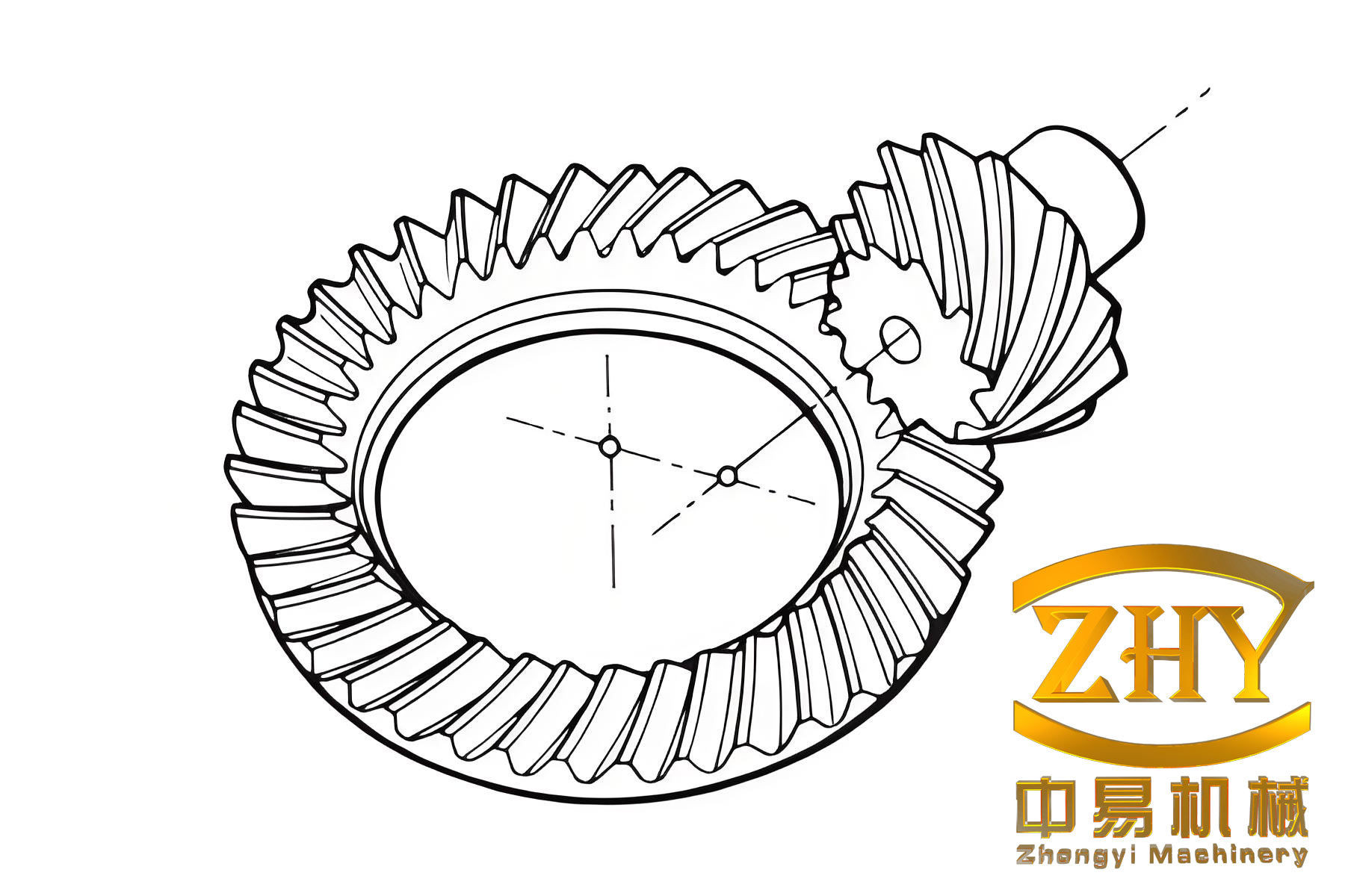
With the mathematical models in place, the next step is to construct a three-dimensional geometric simulation model. I implement the derived equations in a computational environment, such as MATLAB or Python, to generate point clouds for the tooth surfaces and fillet surfaces. These point clouds are then imported into CAD software, where they are used to create smooth surfaces through interpolation or fitting algorithms. The resulting 3D model includes both the gear and pinion, assembled according to their nominal positions. An example of such a model is shown below, where the hypoid bevel gear pair is visualized with an offset of 38 mm and a shaft angle of 90°. The gear is right-handed, and the pinion is left-handed, with the pinion axis positioned below the gear axis (lower offset) to increase pinion diameter and stiffness.
This geometric model serves as the basis for further analysis, including tooth contact analysis (TCA) and loaded tooth contact analysis (LTCA). Before proceeding to LTCA, it is beneficial to perform unloaded TCA to understand the kinematic behavior. In TCA, the meshing of the gear pair is simulated by solving the equations of contact and tangency between the tooth surfaces. The condition for contact is that the position vectors and normal vectors of corresponding points on the gear and pinion surfaces coincide in a fixed coordinate system. Mathematically, this is expressed as:
$$ \mathbf{r}_2(\theta_g, \phi_g, \phi_2) = \mathbf{r}_1(\theta_p, \phi_p, \phi_1), $$
$$ \mathbf{n}_2(\theta_g, \phi_g, \phi_2) = \mathbf{n}_1(\theta_p, \phi_p, \phi_1), $$
where \( \mathbf{r}_2 \) and \( \mathbf{r}_1 \) are the position vectors, and \( \mathbf{n}_2 \) and \( \mathbf{n}_1 \) are the unit normal vectors. By solving these equations along with the meshing conditions, I obtain the transmission error, which is defined as the deviation from ideal uniform motion. The transmission error curve typically shows a parabolic shape under no-load conditions, indicating the inherent flexibility of the gear mesh. For the hypoid bevel gears in this study, the unloaded transmission error is minimal, suggesting good design for noise reduction.
Now, let me move to the core of this work: loaded tooth contact analysis. LTCA simulates the gear pair under actual operating loads, accounting for tooth deflections and contact deformations. The method I use is based on a compliance matrix approach, where the tooth stiffness is represented by a matrix that relates applied loads to displacements. The gear teeth are discretized along potential contact lines, and the compliance of each discrete point is pre-calculated using finite element analysis or analytical formulas. The contact problem under load is formulated as a constrained optimization problem, where the objective is to minimize the strain energy subject to contact conditions. The governing equations are:
$$ \mathbf{F} \mathbf{p} + \mathbf{w} = \theta \mathbf{r} + \mathbf{d}, $$
$$ \mathbf{p}^T \mathbf{r} = T, $$
where \( \mathbf{p} \) is the vector of normal loads at discrete contact points, \( \mathbf{F} \) is the flexibility matrix, \( \mathbf{w} \) is the initial separation vector (including unloaded transmission error and tooth gaps), \( \theta \) is the relative angular displacement due to loading, \( \mathbf{r} \) is the moment arm vector, \( \mathbf{d} \) is the final separation vector, and \( T \) is the applied torque. The contact conditions require that if a point is in contact (\( p_i > 0 \)), the final separation \( d_i = 0 \); if not (\( p_i = 0 \)), then \( d_i > 0 \). This is a nonlinear programming problem that I solve iteratively to find the load distribution and loaded transmission error.
For the hypoid bevel gear pair in this study, I apply a torque of 500 N·m to the gear and perform LTCA. The results include the contact pattern on the tooth surface, the loaded transmission error curve, and the load distribution factor. The contact pattern shows that under this load, the contact area is concentrated in the central region of the tooth, but as the load increases, edge contact may occur. The loaded transmission error curves for different torque levels (e.g., 50, 150, 300, 500 N·m) are plotted, revealing that the error amplitude remains small and smooth, indicating stable transmission. However, at 500 N·m, edge contact is observed, which could lead to increased stress and noise. The load distribution factor indicates that multiple tooth pairs share the load, with a high contact ratio that enhances smoothness. To quantify these results, I present the following table summarizing key LTCA outputs for various torque levels.
| Torque (N·m) | Loaded Transmission Error Peak (arcsec) | Contact Area Size (mm²) | Maximum Contact Pressure (MPa) | Edge Contact Occurrence |
|---|---|---|---|---|
| 50 | 5.2 | 15.3 | 350 | No |
| 150 | 6.8 | 18.7 | 480 | No |
| 300 | 8.5 | 22.1 | 620 | No |
| 500 | 12.3 | 25.5 | 850 | Yes |
The above table highlights how hypoid bevel gears perform under increasing loads. The contact pressure rises with torque, and edge contact becomes a concern at higher loads, which may necessitate design adjustments such as profile modifications or lead crowning. These insights are crucial for ensuring the durability and efficiency of hypoid bevel gears in heavy-duty applications.
To validate the theoretical models and LTCA results, I conduct cutting tests on a physical gear pair. The gears are manufactured using the HGT method on a CNC hypoid generator, with parameters matching those used in the simulation. After cutting, the tooth surfaces are inspected using coordinate measuring machines (CMM) to verify the geometry. Then, the gear pair is assembled in a test rig and subjected to load tests. The contact patterns under load are recorded using marking compounds, and the transmission error is measured with encoders. The experimental results show good agreement with the simulations: the contact pattern is centrally located under light loads but extends toward the edges at 500 N·m, confirming the edge contact prediction. The transmission error measurements also correlate well with the simulated curves, with minor discrepancies due to manufacturing tolerances and assembly deflections. This validation underscores the accuracy of the derived models and the reliability of the LTCA methodology for hypoid bevel gears.
In addition to the core analysis, it is worth discussing the implications of these findings for gear design optimization. The occurrence of edge contact at high loads suggests that the tooth surface geometry could be optimized to distribute loads more evenly. Techniques such as ease-off topography modification can be applied, where the tooth surface is deliberately altered to control the contact path and pressure distribution. The ease-off is defined as the normal deviation between the real tooth surface and a reference surface, and it can be optimized using numerical methods to minimize loaded transmission error and avoid edge contact. The optimization problem can be formulated as:
$$ \min \left( \int (\Delta TE)^2 \, d\phi + \lambda \cdot \max(P_c) \right), $$
where \( \Delta TE \) is the transmission error variation, \( P_c \) is the contact pressure, and \( \lambda \) is a weighting factor. By solving this problem, I can derive modified machine settings that improve performance. This approach is particularly relevant for hypoid bevel gears, where small adjustments in cutting parameters can have significant effects on meshing behavior.
Furthermore, the dynamic behavior of hypoid bevel gears under load is an important consideration for noise and vibration. The loaded transmission error serves as a primary excitation source for gear dynamics. By minimizing its fluctuations through design optimization, I can reduce vibration levels. The dynamic model can be coupled with the LTCA results to predict system response. For instance, the equation of motion for a gear pair can be written as:
$$ I \ddot{\theta} + c \dot{\theta} + k(t) \theta = T(t), $$
where \( I \) is the inertia, \( c \) is the damping coefficient, \( k(t) \) is the time-varying mesh stiffness obtained from LTCA, and \( T(t) \) is the torque. Solving this equation yields the dynamic transmission error, which can be used to assess noise characteristics. This holistic approach, combining static LTCA with dynamic analysis, is essential for developing quiet and reliable hypoid bevel gear drives.
Another aspect to consider is the effect of misalignments on hypoid bevel gear performance. In practical applications, gear pairs often experience misalignments due to assembly errors, shaft deflections, or thermal expansions. These misalignments can alter the contact pattern and increase transmission error. To account for this, I extend the LTCA to include misalignment parameters, such as axial offsets, shaft angle errors, and mounting distances. The tooth surface equations are modified to incorporate these deviations, and the contact analysis is repeated. The results show that misalignments tend to shift the contact toward the tooth edges, exacerbating edge contact and increasing stress. Therefore, in design, it is prudent to include tolerance analysis and possibly introduce flexibility in the housing to accommodate misalignments without compromising performance.
To illustrate the complexity of hypoid bevel gear geometry, let me present a set of key formulas that summarize the surface generation process. These formulas are derived from the coordinate transformations and meshing conditions, and they are essential for anyone working on gear modeling. First, the transformation from the cutter coordinate system to the gear coordinate system involves a series of rotations and translations. The general form of a homogeneous transformation matrix is:
$$ \mathbf{M} = \begin{bmatrix} \mathbf{R} & \mathbf{t} \\ \mathbf{0} & 1 \end{bmatrix}, $$
where \( \mathbf{R} \) is a 3×3 rotation matrix and \( \mathbf{t} \) is a 3×1 translation vector. For the gear, the rotation matrix might include rotations about the cradle axis, the gear axis, and the cutter axis. The specific angles and offsets depend on the machine settings. The meshing condition can be expressed in differential form as:
$$ \frac{\partial \mathbf{r}}{\partial u} \times \frac{\partial \mathbf{r}}{\partial v} \cdot \mathbf{v}^{(12)} = 0, $$
where \( u \) and \( v \) are surface parameters, and \( \mathbf{v}^{(12)} \) is the relative velocity. This condition ensures that the cutter and gear blank maintain contact during generation. By solving these equations numerically, I obtain the tooth surface as a parametric representation.
In terms of computational implementation, I use iterative methods such as Newton-Raphson to solve the nonlinear equations. The algorithm involves initial guesses for the parameters, followed by updates based on Jacobian matrices. For example, to find a point on the tooth surface, I solve:
$$ \mathbf{F}(\mathbf{x}) = \mathbf{0}, $$
where \( \mathbf{x} = [u, \phi]^T \) and \( \mathbf{F} \) includes the surface and meshing equations. The update step is:
$$ \mathbf{x}_{k+1} = \mathbf{x}_k – \mathbf{J}^{-1}(\mathbf{x}_k) \mathbf{F}(\mathbf{x}_k), $$
with \( \mathbf{J} \) being the Jacobian matrix. This process is repeated until convergence, and then the point is transformed to the global coordinate system. By repeating this for a grid of parameters, I generate the point cloud for the entire tooth surface.
Now, let me discuss the significance of the fillet surface in hypoid bevel gears. The fillet is critical for reducing stress concentrations at the tooth root, where bending stresses are highest. The shape of the fillet is determined by the cutter tip arc and the generating motion. A well-designed fillet can significantly enhance the fatigue life of the gear. In my model, the fillet surface is derived separately from the working surface, but it must blend smoothly with it. The transition curve is where the working surface and fillet surface meet, and it is defined by the condition that their normals are collinear. This ensures geometric continuity, which is important for stress flow. The fillet geometry can be optimized by adjusting the cutter tip radius and the machine motions during cutting. For instance, a larger tip radius generally leads to a smoother fillet but may interfere with tooth thickness requirements.
To further elaborate on the loaded contact analysis, I delve into the calculation of the flexibility matrix \( \mathbf{F} \). This matrix represents the compliance of the tooth structure at discrete points along the contact lines. Each element \( F_{ij} \) denotes the displacement at point \( i \) due to a unit load at point \( j \). I compute these compliances using finite element analysis of a detailed gear model. The FE model includes the tooth, rim, and part of the gear body, with appropriate boundary conditions. By applying unit loads at each discrete point and measuring the deflections, I populate the flexibility matrix. Alternatively, analytical formulas based on beam theory can be used for approximation, but for accuracy, FE methods are preferred. The flexibility matrix is symmetric and positive definite, reflecting the reciprocal nature of elastic deformations. In practice, I often use substructuring techniques to reduce computational cost, especially for large-scale models of hypoid bevel gears.
The load distribution results from LTCA provide insights into the sharing of load among multiple tooth pairs. The contact ratio of hypoid bevel gears is typically high due to their spiral teeth, which means that more than one tooth pair is in contact at any time. This enhances smoothness and reduces noise. The load distribution factor \( K_\gamma \) is defined as the ratio of the maximum load on a tooth pair to the average load. For the gear pair in this study, \( K_\gamma \) is around 1.2 under full load, indicating relatively even sharing. However, at the edges of contact, the load may spike, leading to high localized stresses. This is why edge contact is undesirable and should be mitigated through design.
In the context of manufacturing, the HGT method offers flexibility through adjustable parameters such as the cutter tilt, swivel angle, and modified roll. These parameters control the tooth surface geometry and can be tuned to achieve desired contact patterns. For example, increasing the cutter tilt can bias the contact toward the heel or toe of the tooth. The modified roll modifies the relationship between the cradle rotation and the gear rotation, effectively changing the tooth curvature. By optimizing these parameters using the models I developed, I can design hypoid bevel gears with optimal performance characteristics. This optimization can be framed as a multi-objective problem, minimizing transmission error, contact pressure, and sensitivity to misalignments simultaneously.
To summarize the entire process, I present a flow chart of the methodology in textual form. First, derive the tooth surface equations based on machine kinematics. Second, generate point clouds and create a 3D CAD model. Third, perform unloaded TCA to assess kinematic performance. Fourth, conduct LTCA to evaluate behavior under load. Fifth, validate with cutting tests and measurements. Sixth, optimize design parameters based on analysis results. This systematic approach ensures that hypoid bevel gears meet stringent performance requirements.
Looking ahead, there are several avenues for future work. One direction is to integrate thermal effects into the analysis, as hypoid bevel gears in automotive applications often operate under varying temperatures that affect clearances and material properties. Another direction is to explore additive manufacturing for hypoid bevel gears, which could enable complex geometries not feasible with traditional cutting. Additionally, real-time monitoring and adaptive control of gear meshing using sensors could further enhance performance. The models I developed provide a foundation for these advanced studies, emphasizing the versatility and importance of hypoid bevel gears in modern engineering.
In conclusion, through this detailed exploration, I have demonstrated the comprehensive modeling and analysis of hypoid bevel gears using the HGT method. The mathematical derivations, simulation models, and experimental validations collectively contribute to a deeper understanding of their behavior. The key takeaways are the importance of accurate surface generation, the value of loaded tooth contact analysis in predicting real-world performance, and the need for design optimization to avoid edge contact. Hypoid bevel gears, with their unique geometry and capabilities, will continue to be integral to power transmission systems, and ongoing research will further unlock their potential. I hope this article serves as a valuable resource for engineers and researchers working with these fascinating components.