
In modern high-speed and heavy-duty transmission systems, the helical gear is a cornerstone component due to its superior meshing characteristics, higher contact ratio compared to spur gears, and consequently, smoother operation and greater load-bearing capacity. However, the primary failure mode for these components is often tooth surface damage. To ensure reliability and safety, engineers rely on sophisticated analyses such as Tooth Contact Analysis (TCA) and Loaded Tooth Contact Analysis (LTCA) for strength verification and design validation. The accuracy of these analyses is fundamentally limited by the precision of the underlying geometric model. Traditional finite element models, often built from simplified CAD geometries, can introduce significant inaccuracies, leading to unreliable simulation results. This work addresses this critical gap by presenting a high-fidelity reconstruction methodology for helical gear tooth surfaces using Non-Uniform Rational B-Splines (NURBS), with a novel application of the Particle Swarm Optimization (PSO) algorithm to achieve exceptional fitting accuracy, thereby providing a precise geometric foundation for subsequent TCA and LTCA.
The core of our method lies in constructing a parametric, high-order NURBS representation of the complex tooth surface. NURBS surfaces offer a powerful mathematical framework for representing free-form shapes with high smoothness and local controllability, making them ideal for accurately modeling the involute helicoid of a helical gear. A NURBS surface of degree (p, q) is defined by a control net, knot vectors, and weights, expressed as:
$$S(u, v) = \sum_{i=0}^{n} \sum_{j=0}^{m} P_{i,j} R_{i,j}^{(p,q)}(u, v)$$
where \( P_{i,j} \) are the three-dimensional control points, and \( R_{i,j}^{(p,q)}(u, v) \) are the rational basis functions:
$$R_{i,j}^{(p,q)}(u, v) = \frac{w_{i,j} N_{i,p}(u) N_{j,q}(v)}{\sum_{\hat{i}=0}^{n} \sum_{\hat{j}=0}^{m} w_{\hat{i},\hat{j}} N_{\hat{i},p}(u) N_{\hat{j},q}(v)}$$
Here, \( N_{i,p}(u) \) and \( N_{j,q}(v) \) are the p-th and q-th degree B-spline basis functions defined on knot vectors \( U = \{u_0, u_1, …, u_{m_u}\} \) and \( V = \{v_0, v_1, …, v_{m_v}\} \), and \( w_{i,j} \) are the associated weights. The weights provide an additional degree of freedom; increasing the weight of a control point attracts the surface closer to it, allowing for fine-tuning of the surface shape without altering the control polygon.
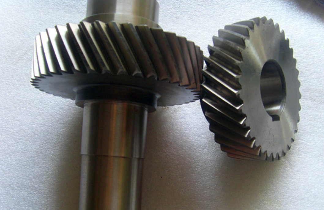
The first step in our reconstruction pipeline is the generation of a high-density point cloud representing the theoretical tooth surface. We derive this from the precise parametric equations of a helical gear. The working flank, an involute helicoid, is generated by sweeping a transverse plane involute along a helical path. Its equation in a coordinate system attached to the gear is given by:
$$
\begin{align*}
x_1(u, \theta) &= r_b \sin(u + \theta) – r_b u \cos(u + \theta) \\
y_1(u, \theta) &= r_b \cos(u + \theta) + r_b u \sin(u + \theta) \\
z_1(u, \theta) &= p \theta
\end{align*}
$$
where \( r_b \) is the base radius, \( \theta \) is the angular parameter of rotation (related to the helix), \( p = r_b / \tan(\beta) \) is the screw parameter, \( \beta \) is the helix angle, and \( u \) is the involute roll angle parameter (\( u = \theta_k + \alpha_k \), with \( \alpha_k \) being the pressure angle at a point).
The fillet (transition) surface, generated by the tip of the hob cutter, is equally critical for stress analysis. Its formulation is more complex, involving the trochoidal path of the hob corner. Its parametric equations can be derived as:
$$
\begin{align*}
x_2(\gamma, \theta) &= r \sin(\phi_1) – \left( \frac{a_1}{\sin \gamma} + \rho \right) \cos \phi_2 \\
y_2(\gamma, \theta) &= r \cos(\phi_1) – \left( \frac{a_1}{\sin \gamma} + \rho \right) \sin \phi_2 \\
z_2(\gamma, \theta) &= p \theta
\end{align*}
$$
with \( \phi_1 = \varphi – \theta \) and \( \phi_2 = \gamma – \varphi + \theta \). Here, \( \gamma \) is a generating parameter, \( \rho \) is the hob tip radius, \( a_1 \) is the distance from the hob corner center to the pitch line, and \( \varphi \) is a phase angle determined by gear and tool geometry. By discretizing these equations over their respective parameter domains, we obtain a structured grid of type points for the involute and fillet surfaces, which serve as the input for the NURBS fitting process. The parameters for the example helical gear studied are summarized in the table below.
| Parameter | Value |
|---|---|
| Number of Teeth, \( z \) | 23 |
| Normal Module, \( m_n \) (mm) | 2 |
| Pressure Angle, \( \alpha_n \) (deg) | 20 |
| Helix Angle, \( \beta \) (deg) | 18 |
| Profile Shift Coefficient, \( x_n \) | 0.3 |
| Face Width (mm) | 38 |
| Tip Diameter (mm) | Calculated |
| Base Diameter, \( d_b \) (mm) | Calculated |
The reconstruction problem is an interpolation/approximation problem: given a set of type points \( Q_{k,l} \) (where \( k=0,…,K \) and \( l=0,…,L \)) sampled from the parametric surface, we must find the control points \( P_{i,j} \), knot vectors \( U, V \), and weights \( w_{i,j} \) of a NURBS surface that accurately represents this data. For a chosen degree (we use cubic, p=q=3), the process begins with parameterization. We assign parameters \( (\bar{u}_k, \bar{v}_l) \) to each type point using the cumulative chord length method, which provides a good distribution reflecting the geometry:
$$
\bar{u}_0 = 0, \quad \bar{u}_k = \bar{u}_{k-1} + \frac{|Q_{k,l} – Q_{k-1,l}|}{\sum_{t=1}^{K} |Q_{t,l} – Q_{t-1,l}|}, \quad \bar{u}_K = 1
$$
This is done for all rows and columns, and averages are taken to form the final parameter sets. The knot vectors are then computed by averaging these node sequences, ensuring the appropriate multiplicity at the ends for endpoint interpolation. With the parameters and knots determined, the B-spline basis functions \( N_{i,p}(\bar{u}_k) \) and \( N_{j,q}(\bar{v}_l) \) can be evaluated for all data points.
The core computational step is the control point inversion. Setting all weights initially to 1, the problem reduces to a B-spline fitting. For a fixed \( v \)-direction parameter \( \bar{v}_l \), the points \( Q_{k,l} \) define a B-spline curve in the \( u \)-direction. We solve for the intermediate control points \( \hat{P}_{i,l} \) of these curves by setting up and solving a linear system for each column \( l \):
$$ Q_{k,l} = \sum_{i=0}^{n} \hat{P}_{i,l} N_{i,p}(\bar{u}_k) $$
Subsequently, these intermediate points \( \hat{P}_{i,l} \) are treated as type points for curves in the \( v \)-direction. Solving another set of linear systems yields the final control net \( P_{i,j} \):
$$ \hat{P}_{i,l} = \sum_{j=0}^{m} P_{i,j} N_{j,q}(\bar{v}_l) $$
This two-step process, executed for the involute, fillet, and tip surfaces separately, generates initial NURBS patches. However, the accuracy of this initial fit, governed primarily by the number and distribution of control points, may be insufficient for high-precision analysis. The critical challenge is to quantify and minimize the fitting error.
Traditional error metrics like the maximum Euclidean distance from the NURBS surface to the type points are computationally intensive and may not reflect the true geometric deviation normal to the ideal surface. For a helical gear, the most relevant error is the normal deviation of the fitted surface from the theoretical involute helicoid, as this directly impacts contact kinematics and stress distribution. Therefore, we define a precise Normal Projection Distance (NPD) error metric. For a point \( \mathbf{S}(u_f, v_f) \) on the fitted NURBS surface, we find its projection onto the theoretical involute surface \( \mathbf{r}(u_t, \theta_t) \) along the latter’s unit normal vector \( \mathbf{n}(u_t, \theta_t) \). The relationship is:
$$ \mathbf{S}(u_f, v_f) – \mathbf{r}(u_t, \theta_t) = \delta \cdot \mathbf{n}(u_t, \theta_t) $$
where \( \delta \) is the sought-after normal distance (error). The unit normal for the involute helicoid derived from the cross product of partial derivatives is:
$$ \mathbf{n}(u_t, \theta_t) = \begin{pmatrix} \cos \beta \cos(u_t + \theta_t + \phi’) \\ -\cos \beta \sin(u_t + \theta_t + \phi’) \\ -\sin \beta \end{pmatrix} $$
Here, \( \phi’ \) is a fixed phase angle for positioning the tooth. This leads to a system of equations that can be solved for the parameters \( (u_t, \theta_t) \) of the projection point and the error \( \delta \). We evaluate this error \( \delta \) for a dense grid of points on the fitted NURBS flank. The overall fitting accuracy is characterized by the peak-to-valley (PV) error:
$$ E_{PV} = \max(\delta) – \min(\delta) $$
This PV error provides a direct, geometrically meaningful measure of the surface reconstruction quality. Our goal is to minimize \( E_{PV} \). Since the initial control point positions \( P_{i,j} \) are fixed by the interpolation conditions, the primary free parameters for minimizing this error are the weights \( w_{i,j} \)** of the control points defining the involute surface. This becomes a high-dimensional, non-linear optimization problem, for which we employ the Particle Swarm Optimization (PSO) algorithm.
PSO is a population-based stochastic optimization technique inspired by the social behavior of bird flocking. In our context, a particle represents a candidate set of weights for the control points of the NURBS involute surface. Each particle \( i \) has a position \( \mathbf{x}_i \) (the vector of all \( w_{i,j} \)) and a velocity \( \mathbf{v}_i \) in the search space. The algorithm proceeds by iteratively updating the velocity and position of each particle based on its own best-known position \( \mathbf{pbest}_i \) and the global best-known position \( \mathbf{gbest} \) found by the entire swarm:
$$ \mathbf{v}_i^{(t+1)} = \omega \mathbf{v}_i^{(t)} + c_1 r_1 (\mathbf{pbest}_i – \mathbf{x}_i^{(t)}) + c_2 r_2 (\mathbf{gbest} – \mathbf{x}_i^{(t)}) $$
$$ \mathbf{x}_i^{(t+1)} = \mathbf{x}_i^{(t)} + \mathbf{v}_i^{(t+1)} $$
Here, \( \omega \) is the inertia weight, \( c_1 \) and \( c_2 \) are acceleration coefficients (typically set to 2.0), and \( r_1, r_2 \) are random numbers in [0,1]. The fitness of a particle, which we aim to minimize, is precisely the PV error \( E_{PV}(\mathbf{x}_i) \) of the NURBS surface generated with the weights defined by \( \mathbf{x}_i \). To balance global exploration and local exploitation, we use a decreasing inertia weight strategy:
$$ \omega^{(t+1)} = \alpha \cdot \omega^{(t)} $$
with \( \alpha \in (0,1) \). This allows the swarm to explore widely initially and then refine the search near promising areas. The optimization workflow is as follows:
- Generate initial NURBS involute surface with all weights = 1.
- Initialize a swarm of particles with random weight vectors within bounds (e.g., [0.9, 1.25]).
- For each particle, construct the corresponding NURBS surface, compute the PV error \( E_{PV} \) over a 50×50 evaluation grid.
- Evaluate fitness, update \( \mathbf{pbest} \) and \( \mathbf{gbest} \).
- Update velocities and positions of all particles according to the PSO equations.
- Repeat steps 3-5 until convergence (minimal fitness improvement) or a maximum iteration count is reached.
The result is an optimized set of weights that minimizes the normal deviation of the fitted NURBS surface from the perfect involute helicoid of the helical gear.
We applied this methodology to the example helical gear. The initial NURBS fitting accuracy is highly dependent on the number of control points. The following table summarizes the PV error for different control point configurations (U x V) for one involute flank, with all weights set to unity.
| Control Point Grid (U x V) | Peak-to-Valley Error \( E_{PV} \) (μm) | Observation |
|---|---|---|
| 6 x 4 | ~15.2 | High error, uneven distribution along face width. |
| 6 x 6 | ~8.7 | Improved, but error still significant. |
| 10 x 4 | ~5.1 | Better, but v-direction control insufficient. |
| 10 x 6 | 2.059 | Error is low and evenly distributed. Chosen for optimization. |
The 10×6 configuration offered a good balance between model complexity (60 control points) and initial accuracy. Even this relatively accurate initial fit had a PV error of 2.059 μm. The PSO algorithm was then deployed to optimize the 60 weight parameters. The algorithm parameters were set as: swarm size = 40, \( c_1 = c_2 = 2.0 \), initial \( \omega = 0.95 \), \( \alpha = 0.98 \), maximum iterations = 40. The convergence plot showed rapid improvement in the first 10 iterations, with the fitness (PV error) stabilizing thereafter.
The optimization was successful, reducing the fitting error substantially. The results before and after PSO optimization are contrasted below:
| Condition | Peak-to-Valley Error \( E_{PV} \) (μm) | Improvement |
|---|---|---|
| Before PSO (Weights=1) | 2.059 | Baseline |
| After PSO Optimization | 1.657 | 19.5% reduction |
This final error of 1.657 μm is exceptionally low. To contextualize, the ISO 1328-1 standard for gear accuracy defines various tolerance grades. The total profile deviation \( F_\alpha \) for a gear of comparable size at quality grade 2 is on the order of a few micrometers. Our reconstructed NURBS surface error falls well within this stringent tolerance band, confirming that the method produces a geometric model suitable for high-precision analysis. The optimized NURBS patches for the involute, fillet, and tip can be seamlessly joined (with G1 or G2 continuity techniques) to form a complete, watertight, and highly accurate digital twin of a single helical gear tooth.
In conclusion, this research presents a comprehensive and robust framework for the high-precision reconstruction of helical gear tooth surfaces. By leveraging the flexibility of NURBS mathematics and enhancing it with an intelligent PSO-based optimization loop targeting the normal projection error, we achieve a level of geometric fidelity that surpasses conventional CAD modeling techniques. The key contributions are: 1) A complete parametric formulation for generating precise type points for the helical gear involute and fillet surfaces. 2) A systematic NURBS surface interpolation procedure suitable for complex gear geometry. 3) The definition of a physically meaningful Normal Projection Distance error metric tailored for gear flanks. 4) The successful integration of the PSO algorithm to optimally tune NURBS control point weights, reducing the PV fitting error by nearly 20% to approximately 1.66 μm. This resulting digital model provides the essential, high-integrity geometric input required for reliable Tooth Contact Analysis and Loaded Tooth Contact Analysis, ultimately leading to more accurate predictions of gear mesh behavior, stress, and fatigue life in the design of advanced transmission systems. Future work may focus on extending the optimization to include control point coordinates and applying this methodology to crowned or deliberately modified helical gear tooth surfaces.