
With the rapid development of new energy vehicles and the increasing demand for energy efficiency, optimizing the transmission system has become a critical research focus. The helical gear is a core component for power transmission, and its power loss characteristics directly impact the overall efficiency and endurance of the vehicle. This study focuses on the helical gear transmission within a pure electric vehicle reducer. I have conducted a detailed simulation and analysis of potential energy losses during the operation of helical gear pairs using Amesim simulation software. The primary objective is to establish a simulation model capable of predicting various loss components and to identify optimal gear parameters that minimize total power dissipation, thereby providing a valuable reference for gear design optimization.
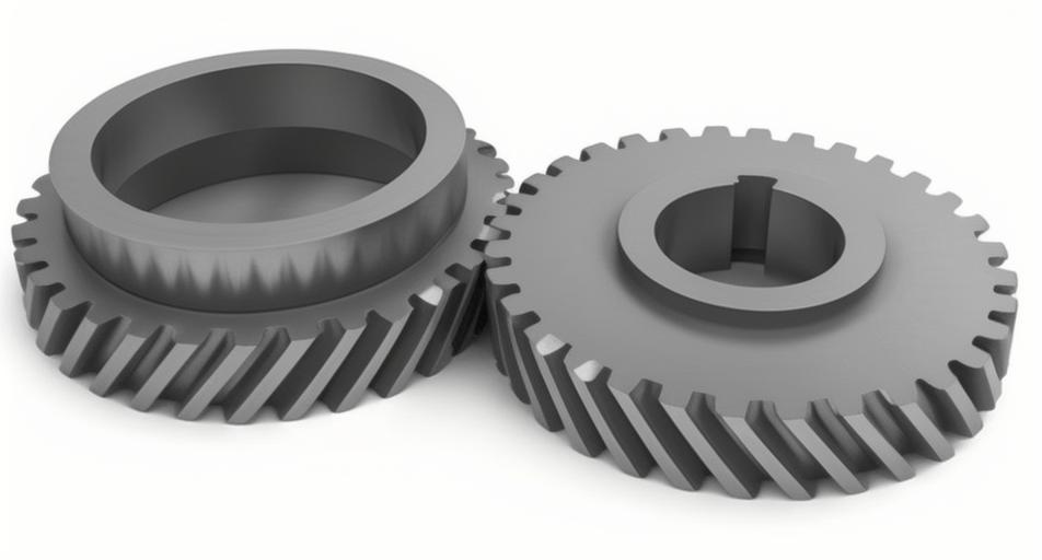
The total power loss in a helical gear transmission system is primarily composed of three major parts: friction losses at the meshing interface, churning losses from the lubricant, and losses originating from the supporting bearings. A comprehensive theoretical model is essential for accurate simulation.
Theoretical Calculation of Helical Gear Power Loss
Friction Power Loss at the Meshing Interface (PF)
Meshing friction loss arises from relative motion between the contacting tooth surfaces. For helical gears, this includes both sliding friction loss (Pf) and rolling friction loss (Pn). The total meshing friction power loss is their sum:
$$P_F = P_f + P_n$$
Sliding Friction Power Loss (Pf): This is dominant and is calculated based on the average normal load \( \bar{F_n} \) and the average sliding velocity \( \bar{v_s} \) at the meshing point.
$$P_f = \frac{\bar{f} \bar{F_n} \bar{v_s}}{1000}$$
where \( \bar{f} \) is the average sliding friction coefficient, empirically estimated as:
$$ \bar{f} = 0.0127 \times \lg\left( \frac{29660 \cdot F_n \cdot \cos \beta}{b \cdot \mu \cdot \bar{v_s} \cdot \bar{v_t}} \right) $$
The normal load \( F_n \) is derived from the input torque \( T \), the pinion pitch radius \( r_1 \), pressure angle \( \alpha \), and helix angle \( \beta \):
$$ F_n = \frac{T}{r_1 \cos \alpha \cos \beta} $$
The average sliding velocity \( \bar{v_s} \) and average rolling velocity \( \bar{v_t} \) are functions of rotational speed \( n \) (in rpm), gear teeth numbers \( z_1, z_2 \), and the length of the path of contact \( g \).
$$ \bar{v_s} = 0.02618 \cdot n \cdot g \cdot \frac{z_1 + z_2}{z_2} $$
$$ \bar{v_t} = 0.2094 \cdot \left[ n \cdot r_1 \cdot \sin \alpha – 0.125 \cdot n \cdot g \cdot \frac{z_1 – z_2}{z_2} \right] $$
Rolling Friction Power Loss (Pn): This occurs under elastohydrodynamic lubrication (EHL) conditions.
$$ P_n = \frac{0.09 \cdot \bar{h} \cdot \bar{v_t} \cdot b \cdot \varepsilon_\alpha}{\cos \beta} $$
Here, \( \bar{h} \) is the average EHL film thickness:
$$ \bar{h} = 2.051 \times 10^{-7} \cdot (\bar{v_t} \mu)^{0.67} \cdot (F_n)^{-0.067} \cdot \rho^{0.464} $$
And \( \varepsilon_\alpha \) is the transverse contact ratio:
$$ \varepsilon_\alpha = \frac{g}{\pi m \cos \alpha} $$
where \( m \) is the module and \( \rho \) is the radius of curvature at the contact point.
Churning (Windage) Power Loss of Helical Gears (PG)
When helical gears rotate partially or fully submerged in lubricant, they must overcome the fluid’s resistance, leading to churning loss. According to the ISO/TR 14179-1 standard, it consists of three components: loss from the smooth outer diameter \( P_{C1} \), loss from a smooth disk \( P_{C2} \), and loss from the tooth faces \( P_{C3} \).
$$ P_G = P_{C1} + P_{C2} + P_{C3} $$
The formulas are as follows:
$$ P_{C1} = \frac{7.37 \cdot f_g \cdot \mu_0 \cdot n^3 \cdot D^{4.7} \cdot L}{A_g \cdot 10^{26}} $$
$$ P_{C2} = \frac{1.474 \cdot f_g \cdot \mu_0 \cdot n^3 \cdot D^{5.7}}{A_g \cdot 10^{26}} $$
$$ P_{C3} = \frac{7.37 \cdot f_g \cdot \mu_0 \cdot n^3 \cdot D^{4.7} \cdot b \cdot R_f}{\tan \beta \cdot A_g \cdot 10^{26}} $$
In these equations, \( f_g \) is the gear immersion factor (0 to 1), \( \mu_0 \) is the dynamic viscosity, \( D \) is the outer diameter of the rotating element, \( L \) is its length, \( b \) is the face width, \( A_g \) is a scaling constant (0.2), and \( R_f \) is a surface roughness coefficient for the gear teeth, given by:
$$ R_f = 7.93 – 4.648 \cdot \frac{m_t}{b} $$
where \( m_t \) is the transverse module.
Power Loss in Supporting Bearings (Pz)
Bearings contribute to power loss through rolling friction, sliding friction, lubricant drag, and seal friction. The new SKF equation provides a comprehensive method to calculate the total frictional torque \( M_{total} \), which is then used to find the power loss.
$$ P_z = \frac{(M_r + M_s + M_d + M_e) \cdot n}{9549} $$
1. Rolling Frictional Torque (Mr): Related to the bearing load.
$$ M_r = G_{r} (v n)^{0.6} $$
\( G_r \) is the rolling friction variable. For a deep groove ball bearing and a roller bearing, it is calculated differently:
For Deep Groove Ball Bearing:
$$ G_{r}^{ball} = R_1 d_m^{1.96} \left( F_r + \frac{R_2 F_a}{\sin[24.6(F_a/C_0)^{0.24}]} \right)^{0.54} $$
For Roller Bearing:
$$ G_{r}^{roller} = R_1 d_m^{2.38} (F_r + R_2 Y F_a)^{0.31} $$
2. Sliding Frictional Torque (Ms):
$$ M_s = f_1 \cdot G_s $$
The sliding friction variable \( G_s \) also has distinct forms for different bearing types.
For Deep Groove Ball Bearing:
$$ G_{s}^{ball} = \left[ S_1 d_m^{-0.145} F_r^{5} + \frac{S_2 d_m^{1.5} F_a^{4}}{\sin[24.6(F_a/C_0)^{0.24}]} \right]^{1/3} $$
For Roller Bearing:
$$ G_{s}^{roller} = S_1 d_m^{0.82} (F_r + S_2 Y F_a) $$
In these formulas, \( R_1, R_2, S_1, S_2 \) are constants dependent on bearing type; \( d_m \) is the bearing mean diameter; \( F_r \) and \( F_a \) are radial and axial loads; \( C_0 \) is the basic static load rating; \( Y \) is the axial load factor; \( v \) is the kinematic viscosity; and \( f_1 \) is a coefficient.
3. Drag Loss Torque (Md) and Seal Friction Torque (Me): These are also calculated based on lubricant properties and seal type according to the SKF model, but their detailed equations are omitted here for brevity.
Modeling and Simulation Based on Amesim
To simulate the power loss dynamics effectively, I constructed a detailed model in Amesim. The model represents a single-stage helical gear reduction system, incorporating the gear pair, two shafts, and two pairs of roller bearings supporting each shaft, mirroring a typical reducer configuration.
Simulation Model Setup
The Amesim model was built using mechanical library components for rotational inertia, stiffness, and damping, coupled with specialized gear and bearing loss models. The core parameters for the helical gear pair are defined in the following table:
| Parameter | Pinion | Gear |
|---|---|---|
| Number of Teeth, z | 18 | 79 |
| Module, m (mm) | 1.75 | 1.75 |
| Face Width, b (mm) | 30 | 30 |
| Pressure Angle, α (°) | 25 | 25 |
| Helix Angle, β (°) | 30 | 30 |
| Addendum Circle Radius (mm) | 17.19 | |
The bearing models were configured with parameters relevant for loss calculation. A common set of bearing parameters used for both sides is summarized below:
| Parameter | Value |
|---|---|
| Mean Diameter, dm (mm) | 40 |
| Friction Coefficient (load-dependent) | 2.5e-4 |
| Friction Coefficient (speed-dependent) | 2 |
| Moment of Inertia (kg·m²) | 1 |
| Viscous Friction Coefficient (N·m/(r/min)) | 0.05 |
A PID speed controller was implemented to drive the input shaft with a defined speed profile, ensuring dynamic analysis. The controller parameters were set with a time step of 1 ms, a proportional gain of 10, and an integral gain of 0.1. Material properties for the gear contact were defined with a Young’s modulus of 2.1e11 Pa and a Poisson’s ratio of 0.3. The simulated speed profile for the input (gear) involved ramps up to 180 rpm, dwells, and reversal to -180 rpm to examine behavior under different conditions.
Simulation Results and Analysis
The simulation successfully decomposed the total power loss into its constituent parts. A key finding was the relative magnitude of sliding versus rolling friction loss at the meshing interface of the helical gear. The results clearly showed that the sliding friction power loss (Pf) was significantly higher than the rolling friction power loss (Pn) throughout the operational cycle. This confirms that sliding friction is the dominant mechanism in gear meshing friction loss for this helical gear setup.
The churning loss components were also captured, differentiating between losses generated by the gear sides and those from the tooth spaces. Similarly, the model computed the comprehensive bearing losses, aggregating the rolling, sliding, drag, and seal friction torques as per the SKF methodology.
To investigate the influence of helical gear geometric parameters on total power loss, I conducted a parametric study. Five different gear configurations were simulated by systematically varying key parameters. The parameter sets are listed below:
| Set # | Gear Teeth (z) | Face Width (mm) | Immersion Depth (mm) | Helix Angle (°) | Pressure Angle (°) |
|---|---|---|---|---|---|
| 1 | 79 | 35 | 55 | 40 | 35 |
| 2 | 58 | 30 | 50 | 30 | 30 |
| 3 | 50 | 25 | 40 | 23 | 25 |
| 4 | 42 | 20 | 35 | 15 | 20 |
| 5 | 36 | 15 | 30 | 5 | 15 |
The simulation results for total power loss across these parameter sets revealed clear trends:
- Number of Teeth (z): Increasing the number of teeth on the driven helical gear led to a decrease in total power loss.
- Face Width (b): Increasing the face width of the helical gear resulted in a significant increase in total power loss, primarily due to increased churning and friction areas.
- Immersion Depth: A deeper immersion of the helical gear in lubricant caused a substantial rise in total power loss, as expected from churning loss models.
- Helix Angle (β): Contrary to some efficiency benefits in load capacity, a larger helix angle for this helical gear configuration increased the total power loss in this simulation context.
- Pressure Angle (α): Increasing the pressure angle of the helical gear contributed to a reduction in the total power loss.
Among the five configurations, Set #5 (with the lowest face width, immersion depth, and helix angle, but a moderate pressure angle and lower tooth count) yielded the lowest total power loss. In contrast, Set #2 resulted in the highest power dissipation. This parametric analysis highlights the complex trade-offs involved in helical gear design for efficiency.
Conclusion
In this study, I developed and validated a simulation model for analyzing power loss in pure electric vehicle reducer helical gears using Amesim software. The model successfully integrates theoretical calculations for meshing friction, churning, and bearing losses into a dynamic simulation framework. By employing the new SKF equation for bearing friction and a PID-based control strategy, the model provides a realistic representation of the helical gear transmission system’s behavior under varying operating conditions.
The simulation results effectively delineate the contributions of different loss mechanisms, confirming that sliding friction is the predominant source of loss at the helical gear meshing interface. Furthermore, the parametric study demonstrates the model’s utility as a design optimization tool. It allows engineers to explore the impact of key helical gear parameters—such as number of teeth, face width, helix angle, pressure angle, and immersion depth—on overall transmission efficiency. Identifying the parameter set that minimizes total loss (Set #5 in this case) provides a direct pathway for improving the energy efficiency of helical gear transmissions. This work establishes a practical methodology for evaluating and optimizing helical gear power losses, contributing valuable insights for the design of more efficient automotive drivetrains.
Future work could involve extending the model to multi-stage gearboxes, incorporating thermal effects on lubricant viscosity and gear deformation, and validating the simulation results against experimental data from a physical helical gear test rig.