
In the realm of precision machinery, the rotary vector reducer has emerged as a pivotal transmission mechanism, integrating planetary gear systems with cycloidal pin wheel configurations to achieve high performance in compact designs. My focus in this investigation is to delve into the deviation sources that critically influence the transmission accuracy of rotary vector reducers. By examining these deviations through a probabilistic lens, I aim to establish a comprehensive modeling framework that enhances our understanding of assembly processes and their impact on overall system reliability. The rotary vector reducer, often abbreviated as RV reducer, is renowned for its advantages such as small size, lightweight construction, high load-bearing capacity, large transmission ratios, longevity, and smooth operation. These attributes make it indispensable in applications like industrial robot joints, CNC machine tools, and aerospace systems, aligning with global initiatives like Industry 4.0 and smart manufacturing trends. However, the transmission precision of rotary vector reducers is susceptible to various deviations arising from manufacturing and assembly, necessitating a thorough analysis to mitigate errors and optimize performance.
The significance of this study stems from the growing demand for high-precision rotary vector reducers in automated systems. While prior research has explored factors affecting transmission accuracy, gaps remain in deviation modeling, particularly in quantifying how multiple error sources interact during assembly. I address this by classifying deviation sources, developing mathematical models using vector and statistical methods, and analyzing deviation propagation mechanisms. This approach not only advances the theoretical foundation for rotary vector reducers but also offers practical insights for quality control in production. Throughout this article, I will frequently refer to the rotary vector reducer to emphasize its central role in our discussion, ensuring that key concepts are tied to this critical component.
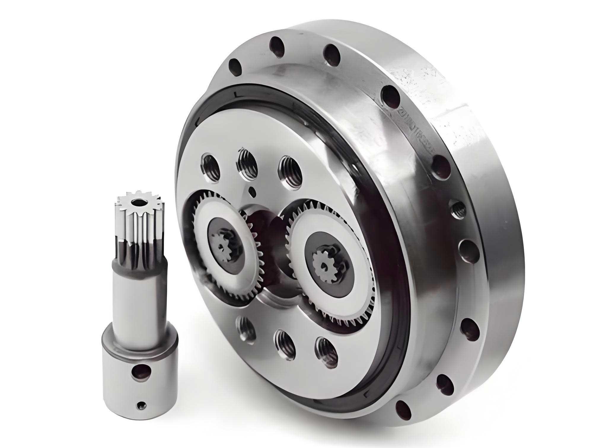
To begin, let me outline the transmission principle of the rotary vector reducer. It consists of a two-stage reduction mechanism: the first stage involves an involute planetary gear system where the sun gear meshes with planet gears to achieve initial speed reduction, and the second stage employs a cycloidal pin wheel system where cycloidal gears engage with fixed pins to further reduce speed and enhance torque. This dual-stage design contributes to the compactness and efficiency of the rotary vector reducer. The core components include the sun gear, planet gears, cycloidal gears, pin housing, crankshafts, and planet carrier, as illustrated in the image above. Understanding this structure is essential for identifying deviation sources, as each part’s geometric and positional inaccuracies can cascade through the assembly, ultimately affecting output precision.
In my analysis, I categorize deviation sources into three primary types, each contributing uniquely to the overall error in rotary vector reducers. These categories are based on static assembly considerations, where deviations are treated as inherent properties of parts and their interactions. Below, I summarize these deviation sources in a table to provide a clear overview:
| Deviation Type | Description | Examples in Rotary Vector Reducers |
|---|---|---|
| Geometric Position Deviation (E1) | Errors in the location and orientation of part features, including linear and angular dimensions. | Diameter variations in crankshafts, parallelism errors between input and output shafts. |
| Geometric Shape Deviation (E2) | Errors in the form or contour of part surfaces, such as straightness or profile deviations. | Cycloidal gear profile inaccuracies, surface flatness of mounting interfaces. |
| Assembly Position Deviation (E3) | Errors arising from part fitting during assembly, including gaps and misalignments due to clearance. | Uncertainties in gear meshing positions, pin housing alignment offsets. |
These deviation sources often couple during assembly, leading to cumulative effects that degrade the transmission accuracy of rotary vector reducers. For instance, a slight geometric shape deviation in a cycloidal gear can amplify when combined with assembly position deviations, resulting in significant backlash or vibration. To model these interactions, I adopt a vector-based approach that represents deviations in a multidimensional space. Each deviation source is expressed as a vector in six degrees of freedom: three linear displacements and three angular rotations. The general form of a deviation vector is given by:
$$ \mathbf{E} = (\Delta u, \Delta v, \Delta w, \Delta \alpha, \Delta \beta, \Delta \gamma) $$
where $\Delta u$, $\Delta v$, and $\Delta w$ denote linear deviations along the x, y, and z axes, respectively, and $\Delta \alpha$, $\Delta \beta$, and $\Delta \gamma$ represent angular deviations around these axes. This representation allows for a unified treatment of various deviation types, facilitating the analysis of their propagation through the assembly of rotary vector reducers.
Next, I define the pose transformation matrix for parts in the rotary vector reducer, which describes how deviations affect part positions and orientations. The transformation combines linear translation and rotation matrices. For a part with deviation vector $\mathbf{E}$, the homogeneous transformation matrix $\mathbf{T}$ is derived as follows. The linear translation matrix is:
$$ \text{Trans} = \begin{pmatrix} 1 & 0 & 0 & \Delta u \\ 0 & 1 & 0 & \Delta v \\ 0 & 0 & 1 & \Delta w \\ 0 & 0 & 0 & 1 \end{pmatrix} $$
and the rotation matrix, assuming small angles for simplicity, is approximated as:
$$ \text{Rot} \approx \begin{pmatrix} 1 & -\Delta \gamma & \Delta \beta & 0 \\ \Delta \gamma & 1 & -\Delta \alpha & 0 \\ -\Delta \beta & \Delta \alpha & 1 & 0 \\ 0 & 0 & 0 & 1 \end{pmatrix} $$
The combined transformation matrix $\mathbf{T}$ is then $\mathbf{T} = \text{Trans} \times \text{Rot}$. This matrix is crucial for simulating how deviations accumulate across multiple parts in a rotary vector reducer. For example, if a crankshaft has a geometric position deviation, its transformed pose can affect the meshing of cycloidal gears, leading to transmission errors. By applying these matrices sequentially for each part, I can model the overall deviation stack-up in the assembly process.
To incorporate probabilistic aspects, I assume that each component of the deviation vector follows a normal distribution. This is reasonable in manufacturing contexts where variations tend to cluster around nominal values. For a deviation vector $\mathbf{E}$, the linear and rotational components are modeled as:
$$ \Delta u \sim N(\mu_1, \sigma_1^2), \quad \Delta v \sim N(\mu_2, \sigma_2^2), \quad \Delta w \sim N(\mu_3, \sigma_3^2) $$
$$ \Delta \alpha \sim N(\mu_4, \sigma_4^2), \quad \Delta \beta \sim N(\mu_5, \sigma_5^2), \quad \Delta \gamma \sim N(\mu_6, \sigma_6^2) $$
Here, $\mu_i$ represents the mean deviation, and $\sigma_i^2$ denotes the variance for each degree of freedom. The multivariate statistical model for the deviation vector is given by the probability density function:
$$ f(\mathbf{E}) = (2\pi)^{-3} |\mathbf{P}|^{-1/2} \exp\left(-\frac{1}{2} (\mathbf{E} – \boldsymbol{\mu})^T \mathbf{P}^{-1} (\mathbf{E} – \boldsymbol{\mu})\right) $$
where $\boldsymbol{\mu} = (\mu_1, \mu_2, \mu_3, \mu_4, \mu_5, \mu_6)$ is the mean vector, and $\mathbf{P}$ is the covariance matrix capturing correlations between deviation components. For instance, in a rotary vector reducer, the diameter deviation of a shaft might correlate with its straightness error, influencing the covariance structure. This model enables a statistical evaluation of deviation magnitudes, which is essential for predicting the likelihood of exceeding tolerance limits in rotary vector reducers.
Now, let me elaborate on the concept of deviation domains, which define the permissible ranges for deviations. A deviation domain is a spatial region bounded by tolerance limits, and it aligns with the geometric coordinate system of the part. For rotary vector reducers, common deviation domains include parallel plane domains and cylindrical domains. As an example, consider a parallel plane domain for a flat surface, where the linear deviation $\Delta w$ is constrained between two planes separated by a tolerance $\Delta t$. The angular deviations $\Delta \alpha$ and $\Delta \beta$ are limited by the surface dimensions $L_1$ and $W_1$. The constraints can be expressed as:
$$ |\Delta w| \leq \Delta t, \quad |\Delta \alpha| \leq \frac{2\Delta t}{L_1}, \quad |\Delta \beta| \leq \frac{2\Delta t}{W_1} $$
with $\Delta u = \Delta v = \Delta \gamma = 0$ for this simple case. The mean vector and covariance matrix for such a domain can be derived based on these bounds. For instance, assuming a uniform distribution within the domain, the mean linear deviation $\mu_3$ is $(\Delta t)/2$, and the variance $\sigma_3^2$ is $(\Delta t)^2/12$. However, in practice, I often use normal approximations for computational efficiency in rotary vector reducer analyses.
To evaluate the impact of each deviation source, I define metrics for linear and rotational deviations. For geometric position deviation $\mathbf{E}_1$, the linear deviation magnitude is computed using the Euclidean norm, weighted by effective radii for angular terms:
$$ \|e(\mathbf{E}_1)\| = \sqrt{(\Delta u)^2 + (\Delta v)^2 + (\Delta w)^2 + (\Delta \alpha)^2 r_\alpha^2 + (\Delta \beta)^2 r_\beta^2 + (\Delta \gamma)^2 r_\gamma^2} $$
where $r_\alpha, r_\beta, r_\gamma$ are the effective radii converting angular deviations to linear equivalents at critical points in the rotary vector reducer. Similarly, the rotational deviation magnitude is:
$$ \|\varepsilon(\mathbf{E}_1)\| = \sqrt{\frac{(\Delta u)^2}{r_\alpha^2} + \frac{(\Delta v)^2}{r_\beta^2} + \frac{(\Delta w)^2}{r_\gamma^2} + (\Delta \alpha)^2 + (\Delta \beta)^2 + (\Delta \gamma)^2} $$
For geometric shape deviation $\mathbf{E}_2$, I first fit a nominal geometry to measurement points. For a plane surface, the fitting error $e_2$ is the average distance from points to the fitted plane, and this error is incorporated into the deviation metrics. For assembly position deviation $\mathbf{E}_3$, the evaluation is similar but focuses on the uncertainties introduced by fitting gaps. These metrics allow me to quantify the contribution of each deviation type to the overall error in rotary vector reducers.
The propagation of deviations through the assembly of a rotary vector reducer is a critical aspect of this study. I analyze deviation transfer mechanisms using directed graphs, where nodes represent part geometries and edges denote deviation flows. Based on the three deviation types, I define five basic deviation flow models, as summarized in the table below:
| Deviation Flow Type | Description | Application in Rotary Vector Reducers |
|---|---|---|
| f1: Same-part geometric position deviation | Deviation between two geometries on the same part due to E1. | Misalignment between crankshaft bearing seats. |
| f2: Geometric shape deviation | Deviation from nominal form due to E2. | Cycloidal gear profile errors affecting meshing. |
| f3: Between-part geometric position deviation | Deviation between geometries on different parts due to E1. | Sun gear to planet gear center distance errors. |
| f4: Assembly position deviation correction | Modification of f3 due to E3 from fitting gaps. | Pin housing alignment adjustments during assembly. |
| f5: Multiple deviation interactions | Combined effects of multiple deviations on a single geometry. | Cumulative errors in planet carrier holes. |
These deviation flows help visualize how errors accumulate in rotary vector reducers. For instance, in a non-clearance fit, deviations propagate continuously from one part to another through geometric constraints, whereas in a clearance fit, the propagation is discontinuous due to gaps, requiring re-initialization of deviation accumulation. The interaction between fit types—such as Mgg (both geometries are deviation-prone), MDD (both are datum geometries), and MgD (mixed)—further complicates the propagation. I model this using state transitions in the directed graph, where each edge weight represents the deviation magnitude transferred.
To illustrate the practical application of these models, consider a shaft-hole fitting assembly in a rotary vector reducer, such as the connection between a crankshaft and a bearing housing. This is an MgD-type fit with clearance. The deviation vector for the assembly can be expressed as $\mathbf{E} = \mathbf{T}_2 + \mathbf{d}_2$, where $\mathbf{T}_2$ is the assembly position deviation and $\mathbf{d}_2$ is the geometric deviation of the hole. Assuming normal distributions for both, the combined deviation is evaluated probabilistically. For example, let the shaft diameter be $d_1 = 25^{+0.10}_{-0.00}$ mm and the hole diameter be $d_2 = 25^{+0.00}_{-0.15}$ mm. In a 3D coordinate system, the maximum linear deviation from the size difference is 0.25 mm, but after probabilistic aggregation, the linear deviation magnitude is computed as approximately 0.4970 mm, and the rotational deviation magnitude is 0.0269 mm. Using trigonometric similarity, the angular error $\Delta \theta$ is about 0.0573°, which aligns with tolerance requirements for rotary vector reducers. This example confirms that my model can effectively analyze deviation accumulation in real assemblies.
Expanding on the statistical model, I derive the covariance matrix for a parallel plane deviation domain. Given tolerance limits $t_1$ and $t_2$ with $\Delta t = t_2 – t_1$, and surface dimensions $L_1$ and $W_1$, the mean vector and covariance matrix are as follows. The mean vector is:
$$ \boldsymbol{\mu} = \left(0, 0, \frac{\Delta t}{2}, \frac{\Delta t}{2L_1}, \frac{\Delta t}{2W_1}, 0\right) $$
and the covariance matrix $\mathbf{P}$ is:
$$ \mathbf{P} = \begin{pmatrix} 0 & 0 & 0 & 0 & 0 & 0 \\ 0 & 0 & 0 & 0 & 0 & 0 \\ 0 & 0 & \sigma_3^2 & \sigma_{34} & \sigma_{35} & 0 \\ 0 & 0 & \sigma_{34} & \sigma_4^2 & 0 & 0 \\ 0 & 0 & \sigma_{35} & 0 & \sigma_5^2 & 0 \\ 0 & 0 & 0 & 0 & 0 & 0 \end{pmatrix} $$
where $\sigma_3^2 = (\Delta t)^2/12$, $\sigma_4^2 = (\Delta t)^2/(3L_1^2)$, $\sigma_5^2 = (\Delta t)^2/(3W_1^2)$, and covariances $\sigma_{34}$ and $\sigma_{35}$ are derived from the constraint relationships. This matrix is used in the multivariate normal distribution to simulate deviation scenarios for rotary vector reducer components.
Furthermore, I investigate the effect of assembly sequences on deviation propagation. In a rotary vector reducer, the order of part installation—such as mounting cycloidal gears before the pin housing—can alter the final deviation accumulation. I model this using sequential transformation matrices, where the pose of each part is updated based on previous assemblies. For a series of $n$ parts, the overall deviation transformation is:
$$ \mathbf{T}_{\text{total}} = \prod_{i=1}^{n} \mathbf{T}_i $$
where $\mathbf{T}_i$ is the transformation matrix for part $i$ including its deviations. This product accounts for both linear and rotational couplings, which are particularly significant in the compact design of rotary vector reducers. For instance, a small angular deviation in the sun gear can amplify through the planetary stage, causing substantial output errors. By simulating different assembly sequences, I can identify optimal strategies to minimize transmission inaccuracies.
Another key aspect is the classification of deviation effects as positive, negative, or uncorrelated in terms of their contribution to overall error. Drawing an analogy to electrical circuits, I use a loop method to determine the sign of deviation accumulation in dimensional chains. For a closed loop representing the output accuracy of a rotary vector reducer, I traverse the chain and assign directions to deviations; those opposing the closed-loop direction are positive accumulators (increasing error), while those aligning are negative accumulators (compensating error). This helps in designing tolerance stacks that balance errors, enhancing the reliability of rotary vector reducers.
In addition to theoretical modeling, I consider practical implications for manufacturing rotary vector reducers. The deviation models developed here can be integrated into computer-aided design (CAD) and computer-aided manufacturing (CAM) systems to predict and compensate for errors. For example, by inputting tolerance data from part drawings, my model can simulate the expected transmission error distribution, allowing engineers to adjust tolerances or assembly processes proactively. This is crucial for high-volume production of rotary vector reducers, where consistency is paramount.
To enhance the robustness of my analysis, I explore sensitivity analysis techniques. By varying the parameters of the deviation distributions—such as means and variances—I assess how changes in manufacturing precision affect the final output of rotary vector reducers. This involves computing partial derivatives of the transmission error with respect to each deviation component. For instance, the sensitivity of the output rotation error $\Delta \theta_{\text{out}}$ to a crankshaft diameter deviation $\Delta d$ can be expressed as:
$$ S = \frac{\partial \Delta \theta_{\text{out}}}{\partial \Delta d} $$
High sensitivity indicates that tight control over that parameter is essential for maintaining accuracy in rotary vector reducers. I compile these sensitivities into a matrix to prioritize quality control measures.
Moreover, I extend the deviation modeling to dynamic conditions, although the focus remains on static assembly. In operation, rotary vector reducers experience loads and thermal effects that may exacerbate deviations. Future work could integrate my static models with dynamic simulations to predict performance under real-world conditions. This would further solidify the role of deviation analysis in optimizing rotary vector reducers for demanding applications like robotics and aerospace.
In conclusion, my investigation into deviation modeling for rotary vector reducers has yielded a comprehensive framework based on probability theory. By classifying deviation sources into geometric position, shape, and assembly position categories, and by developing vector-based and statistical models, I have provided a method to quantify and propagate errors through the assembly process. The use of directed graphs and transformation matrices facilitates the analysis of deviation accumulation, while practical examples validate the model’s effectiveness. This work not only advances the theoretical understanding of rotary vector reducers but also offers actionable insights for improving manufacturing precision. As the demand for high-performance rotary vector reducers grows, such models will be instrumental in achieving the accuracy and reliability required for advanced mechanical systems.
To summarize the key equations and concepts, I present the following table as a quick reference for the deviation modeling approach applied to rotary vector reducers:
| Concept | Mathematical Representation | Application Example |
|---|---|---|
| Deviation Vector | $\mathbf{E} = (\Delta u, \Delta v, \Delta w, \Delta \alpha, \Delta \beta, \Delta \gamma)$ | Representing crankshaft misalignment in a rotary vector reducer. |
| Transformation Matrix | $\mathbf{T} = \text{Trans} \times \text{Rot}$ | Simulating pose changes of cycloidal gears due to errors. |
| Multivariate Normal Model | $f(\mathbf{E}) = (2\pi)^{-3} |\mathbf{P}|^{-1/2} \exp\left(-\frac{1}{2} (\mathbf{E} – \boldsymbol{\mu})^T \mathbf{P}^{-1} (\mathbf{E} – \boldsymbol{\mu})\right)$ | Statistical analysis of tolerance stacks in rotary vector reducer assemblies. |
| Deviation Magnitude | $\|e(\mathbf{E})\| = \sqrt{(\Delta u)^2 + \ldots + (\Delta \gamma)^2 r_\gamma^2}$ | Quantifying overall error contribution from a planet gear. |
| Sensitivity Analysis | $S = \frac{\partial \Delta \theta_{\text{out}}}{\partial \Delta d}$ | Evaluating impact of pin housing diameter on output accuracy. |
This comprehensive analysis underscores the importance of deviation modeling in the design and production of rotary vector reducers. By leveraging probability theory and advanced mathematical tools, I have established a foundation for enhancing transmission precision, which is critical for the evolving needs of modern industry. The rotary vector reducer, as a key component in precision drives, benefits immensely from such detailed scrutiny, paving the way for more reliable and efficient mechanical systems in the future.