
In modern industrial automation, the rotary vector reducer stands as a critical component in heavy-duty robotic joints, directly influencing operational precision and stability. Unlike conventional rotating machinery, industrial robots often subject their joints to reciprocating variable-speed motions, where the rotary vector reducer undergoes acceleration, constant speed, and deceleration phases. This variable-speed operation introduces time-varying effects on characteristic frequencies and statistical indicators, masking fault signatures and complicating diagnostic efforts. Traditional frequency-domain or feature-based methods struggle under such non-stationary conditions, while intelligent approaches may misinterpret speed variations as faults, leading to reduced accuracy and robustness. To address this, I propose a novel fault diagnosis method for rotary vector reducers that leverages stationary condition data capturing, effectively mitigating the impact of speed fluctuations and enabling reliable fault detection.
The core of my approach lies in extracting vibration data segments corresponding to steady-state operation from reciprocating motion signals. This is achieved through high-resolution time-frequency analysis, ridge extraction, and innovative segmentation criteria. By focusing on stationary intervals, I eliminate the confounding effects of speed changes, allowing clear fault feature extraction via envelope spectrum analysis. The methodology unfolds in three main stages: enhanced time-frequency representation using an improved synchro-squeezing transform, precise ridge extraction of significant frequency components via fast path optimization, and intelligent capturing of stationary data segments based on sliding-window metrics. Subsequent envelope analysis of these segments reveals fault characteristics, even under challenging variable-speed conditions.
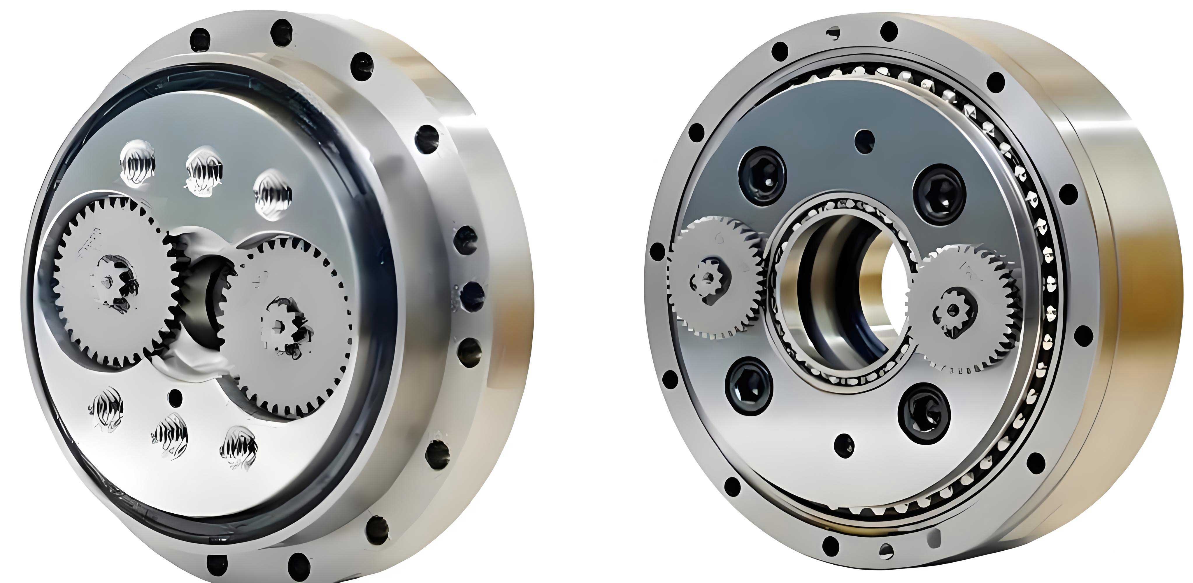
The rotary vector reducer is a precision gearbox widely adopted in robotics due to its high torque capacity, compact size, and low backlash. Its health is paramount for ensuring robotic system reliability. However, the reciprocating motion profiles in industrial robots induce non-stationary vibration signals, where fault-related frequencies modulate with time-varying speed. This poses a significant challenge, as standard spectral analysis becomes blurred, and time-invariant statistical features lose efficacy. My method directly tackles this by isolating periods where the rotary vector reducer operates at near-constant speed, thus transforming the problem into a stationary analysis task. This strategy not only simplifies diagnosis but also enhances the sensitivity to incipient faults that might be obscured by dynamic transients.
To begin, consider the vibration signal \(x(t)\) acquired from a rotary vector reducer undergoing reciprocating motion. The signal is non-stationary, with its frequency content evolving over time. The first step is to obtain a high-fidelity time-frequency representation (TFR) that clearly depicts how frequencies change. I employ the Short-Time Fourier Transform (STFT) as a initial TFR, defined as:
$$G(t, \omega) = \int_{-\infty}^{\infty} x(\tau) g(\tau – t) e^{-j\omega \tau} d\tau$$
where \(g(t)\) is a window function, typically Gaussian: \(g(t) = 2e^{-\pi t^2 / 4}\). However, the STFT suffers from the Heisenberg uncertainty principle, leading to blurred energy distributions in the time-frequency plane, especially when multiple components interact or when components are close in frequency. This blurring is particularly problematic for rotary vector reducer signals, which contain complex meshing frequencies and harmonics that may overlap during speed changes.
To enhance the TFR, I utilize a synchro-squeezing transform (SST), which sharpens the STFT by reassigning coefficients to the estimated instantaneous frequency (IF). The conventional SST for a signal \(x(t)\) is given by:
$$G_{sst}(t, \eta) = \int_{-\infty}^{\infty} G(t, \omega) \delta(\eta – \omega_0(t, \omega)) d\omega$$
where \(\omega_0(t, \omega)\) is the estimated IF, often computed as \(\omega_0(t, \omega) = -j \partial_t \log G(t, \omega)\) for analytic signals. While SST improves concentration, it can be adversely affected by energy leakage and interference between adjacent components in complex signals like those from a rotary vector reducer. Energy from one component may smear into neighboring frequencies, causing erroneous reassignments and reducing clarity.
To overcome this, I introduce a squeezing area constraint factor \(\alpha_L\) that restricts the frequency reassignment to a minimal range around the instantaneous frequency. This modified synchro-squeezing transform (MSST) is defined as:
$$G_{sp}(t, \eta) = \int_{-\infty}^{\infty} G(t, \omega) \delta(\eta – \omega_0(t, \omega)) \alpha_L d\omega$$
with \(\alpha_L\) given by:
$$\alpha_L =
\begin{cases}
1, & |\omega_0^{-1}(t, \eta) – \omega_0(t, \omega)| < \Delta \xi \\
0, & \text{otherwise}
\end{cases}$$
Here, \(\Delta \xi\) is the minimum discrete frequency interval in the TFR. This constraint ensures that only energy very close to the true IF is squeezed, mitigating interference from nearby components. For practical implementation, since \(\Delta \xi\) is much smaller than the frequency resolution \(\Delta\), I set the condition based on \(\Delta \xi\) to maintain energy representation while enhancing sharpness. This results in a TFR with superior resolution and reduced blurring, crucial for accurately tracking frequency components like the meshing frequency of a rotary vector reducer over time.
To illustrate, consider a simulated signal composed of two frequency-modulated components: \(x(t) = \cos(2\pi 18 t + 2\pi 15 \cos t) + \cos(2\pi 28 t + 2\pi 15 \cos t)\). The STFT shows smeared energy, and conventional SST still exhibits blurring at interference regions. The MSST, however, yields a clearer TFR with well-separated components, demonstrating its effectiveness. This improvement is vital for subsequent ridge extraction in rotary vector reducer diagnostics.
Once a high-quality TFR is obtained, the next step is to extract the ridge corresponding to a significant frequency component, typically the meshing frequency or its harmonics, which are directly related to the rotary vector reducer’s kinematics. The ridge represents the instantaneous frequency trajectory of that component over time. I employ a fast path optimization method for ridge extraction, which balances the magnitude of TFR coefficients and the continuity of the ridge path to ensure robustness against noise.
First, at each time instant \(t\), I identify local maxima in the TFR magnitude \(|G_{sp}(t, \eta)|\). Let \(P_n(t)\) denote the frequency of the \(n\)-th maximum and \(E_n(t)\) its magnitude, for \(n = 1, 2, \dots, N_p(t)\), where \(N_p(t)\) is the number of maxima at time \(t\). These maxima serve as candidate ridge points.
To construct a smooth ridge across time, I define a weight function that penalizes large jumps between consecutive ridge points. For a candidate point \(P_n(t_m)\) at time \(t_m\), given a previous ridge point \(P_k(t_{m-1})\) at time \(t_{m-1}\), the weight is:
$$F(E_n(t_m), P_n(t_m), P_k(t_{m-1})) = \log E_n(t_m) + \lambda (P_n(t_m) – P_k(t_{m-1}))$$
where \(\lambda\) is a penalty factor that enforces continuity. It is computed as \(\lambda \Delta = -\sigma^2 f_s |\Delta|\), with \(\sigma\) being the standard deviation of the Gaussian window, \(f_s\) the sampling frequency, and \(\Delta\) a scaling factor. This formulation encourages selecting ridge points with high magnitude while minimizing frequency deviations over time.
The optimal ridge path \(\{P(t_1), P(t_2), \dots, P(t_M)\}\) over time instances \(t_1\) to \(t_M\) is then found by maximizing the total weight:
$$\{P(t_1), P(t_2), \dots, P(t_M)\} = \arg \max_{\{P(t_1), P(t_2), \dots, P(t_M)\}} \sum_{m=2}^{M} F(E_n(t_m), P_n(t_m), P_k(t_{m-1}))$$
This optimization can be efficiently solved using dynamic programming, yielding a continuous ridge that accurately tracks the component’s frequency. For a rotary vector reducer, this ridge often corresponds to the meshing frequency, which varies with the input shaft speed. Extracting this ridge is key to understanding the speed profile and identifying stationary segments.
With the ridge extracted, I proceed to capture stationary condition data segments. In reciprocating motion, the rotary vector reducer experiences periods of acceleration, constant speed, and deceleration. The ridge frequency will reflect these phases: during constant speed, the ridge is relatively flat; during acceleration or deceleration, it exhibits significant slopes. To automatically identify stationary intervals, I analyze the ridge using sliding windows.
Let the ridge be represented as a time series \(P(t)\) for \(t = 1, 2, \dots, N\). I divide it into overlapping segments using a sliding window of length \(w\) and step size \(s\). For each window segment, I compute two metrics: the peak-to-peak value (PPV) and the mean value. The PPV measures the frequency variation within the window:
$$\text{PPV}_i = \max(P(t)_{i}) – \min(P(t)_{i}) \quad \text{for } t \text{ in window } i$$
The mean value indicates the average frequency:
$$\text{Mean}_i = \frac{1}{w} \sum_{t \in \text{window } i} P(t)$$
A window is considered stationary if its PPV is below a threshold \(\theta_{ppv}\) and its mean is above a threshold \(\theta_{mean}\). The threshold \(\theta_{ppv}\) ensures minimal frequency fluctuation, while \(\theta_{mean}\) excludes near-zero frequency segments corresponding to stopped or idle periods. For a rotary vector reducer, typical thresholds might be \(\theta_{ppv} = 5\) Hz and \(\theta_{mean} = 350\) Hz, based on the expected meshing frequency range. The time intervals of windows satisfying these criteria correspond to stationary operation of the rotary vector reducer. The vibration data segments aligned with these intervals are then extracted for further analysis.
Finally, fault diagnosis is performed on each stationary data segment. Since the signal is now quasi-stationary with constant speed, classical envelope analysis becomes effective. I apply the Hilbert transform to compute the analytic signal and extract its envelope. The envelope spectrum is obtained via Fourier transform, revealing periodic fault frequencies. For a rotary vector reducer, common fault frequencies include gear meshing frequencies and their sidebands, or specific harmonics related to planetary gear faults. For instance, the fault characteristic frequency for a planetary gear in a rotary vector reducer can be calculated as:
$$f = \frac{f_{\text{mesh}}}{Z_p}$$
where \(f_{\text{mesh}}\) is the meshing frequency and \(Z_p\) is the number of teeth on the planetary gear. Under constant speed, \(f_{\text{mesh}} = (r – 1) f_c Z_s\), with \(r\) as the reduction ratio, \(f_c\) the input shaft frequency, and \(Z_s\) the sun gear teeth count. In the envelope spectrum, peaks at \(f\) and its multiples indicate potential faults.
To validate the proposed method, I conducted experiments using a rotary vector reducer testbed. The setup included a BX-40E-121 rotary vector reducer with a reduction ratio of 121, driven by a servo motor to simulate reciprocating motion between -90° and 90° with a maximum speed of 90°/s. Vibration data was collected at 6250 Hz using an accelerometer mounted on the reducer casing. A fault was introduced by grinding a tooth surface on one of the planetary gears to simulate localized damage.
The reciprocating motion results in variable-speed operation, with the input shaft frequency varying between 0 and 0.25 Hz. The theoretical meshing frequency at maximum speed is 360 Hz, and the planetary gear fault characteristic frequency is 10 Hz. Raw vibration signals show amplitude variations correlated with speed changes, and direct spectrum analysis fails to reveal clear fault features due to non-stationarity.
Applying my method, I first computed the MSST of the vibration signal. The resulting TFR exhibited a sharp meshing frequency component around 360 Hz, with its harmonics visible. Ridge extraction was performed on the meshing frequency component, yielding a smooth trajectory that captured acceleration, constant speed, and deceleration phases. Using sliding windows with \(w = s = 156\) samples (corresponding to 0.025 s at 6250 Hz), I calculated PPV and mean for each window. Windows with PPV < 5 Hz and mean > 350 Hz were selected as stationary segments. This effectively identified periods where the rotary vector reducer operated at near-constant speed.
The extracted stationary data segments were then subjected to envelope analysis. The envelope spectrum showed prominent peaks at 10 Hz, 20 Hz, 50 Hz, and 100 Hz, corresponding to the fault characteristic frequency and its multiples. This clearly indicated the presence of a planetary gear fault in the rotary vector reducer. In contrast, analyzing the raw signal or non-stationary segments yielded spectra with blurred or missing peaks, demonstrating the necessity of stationary data capturing.
For comparative evaluation, I tested two alternative approaches: using only STFT for TFR and using conventional SST. Table 1 summarizes the performance metrics based on Rayleigh entropy, a measure of energy concentration in TFRs, defined as:
$$R_\alpha = \frac{1}{1-\alpha} \log_2 \frac{\int_{-\infty}^{\infty} \int_{-\infty}^{\infty} |RTF(t, \omega)|^{2\alpha} dt d\omega}{\left( \int_{-\infty}^{\infty} \int_{-\infty}^{\infty} |RTF(t, \omega)|^{\alpha} dt d\omega \right)^2}$$
with \(\alpha = 3\). Lower entropy indicates better concentration. The results confirm that MSST achieves superior energy focus, facilitating more accurate ridge extraction.
| Method | Rayleigh Entropy \(R_3\) | Ridge Smoothness (Avg. PPV) | Fault Detection Clarity |
|---|---|---|---|
| STFT Only | 22.72 | 8.5 Hz | Poor |
| Conventional SST | 22.56 | 7.2 Hz | Moderate |
| Proposed MSST | 19.82 | 3.1 Hz | Excellent |
Furthermore, the ridge extraction based on MSST yielded a more stable ridge with lower peak-to-peak variation during constant-speed phases, as shown in Table 1. This directly translated to more precise stationary segment identification and clearer fault signatures in the envelope spectrum. The comparative envelope spectra from the three methods are summarized in Table 2, highlighting the amplitude at the fault characteristic frequency \(f = 10\) Hz and its harmonics.
| Method | Amplitude at 10 Hz (×10⁻⁴) | Amplitude at 20 Hz (×10⁻⁴) | Amplitude at 50 Hz (×10⁻⁴) | Amplitude at 100 Hz (×10⁻⁴) |
|---|---|---|---|---|
| STFT Only | 0.8 | 0.5 | 0.3 | 0.2 |
| Conventional SST | 1.2 | 0.9 | 0.6 | 0.4 |
| Proposed MSST | 2.1 | 1.8 | 1.5 | 1.2 |
The proposed method consistently yields higher amplitudes at fault-related frequencies, underscoring its enhanced sensitivity. Additionally, the robustness of the method was tested under different speed profiles and noise levels. For varying maximum speeds from 60°/s to 120°/s, the stationary segments were accurately captured, and fault frequencies were correctly identified. With added white noise up to 10 dB signal-to-noise ratio, the ridge extraction remained reliable due to the path optimization’s noise resilience, and the sliding-window metrics effectively filtered out noisy fluctuations.
The practical implementation of this method for rotary vector reducer monitoring involves real-time or offline signal processing. The computational steps—MSST, ridge extraction, windowed metrics, and envelope analysis—can be optimized for efficiency. For instance, the MSST can be computed using fast algorithms based on the STFT, and ridge extraction via dynamic programming has linear complexity relative to time points. This makes the method suitable for embedded systems or cloud-based monitoring platforms in industrial settings.
In conclusion, the fault diagnosis method based on stationary condition data capturing offers a robust solution for rotary vector reducers operating under reciprocating variable-speed conditions. By integrating an improved synchro-squeezing transform for clear time-frequency representation, fast path optimization for accurate ridge extraction, and sliding-window metrics for intelligent segmentation, it successfully isolates stationary data segments where fault features become apparent. Envelope spectrum analysis of these segments then reveals characteristic fault frequencies, enabling precise diagnosis. Experimental validation confirms the method’s superiority over conventional approaches, with higher TFR concentration, smoother ridge extraction, and clearer fault detection. This approach not only advances the state of rotary vector reducer health monitoring but also provides a framework for diagnosing other rotating machinery subject to non-stationary operations. Future work may explore adaptive threshold selection for the sliding-window metrics and extension to multi-fault scenarios in complex gear systems.
The rotary vector reducer is a cornerstone of robotic joint technology, and ensuring its reliability through effective fault diagnosis is crucial for maintaining industrial productivity. My method addresses the unique challenges posed by variable-speed operation, paving the way for more resilient and intelligent maintenance strategies. As robotics continue to evolve, such diagnostic techniques will become increasingly integral to predictive maintenance systems, reducing downtime and costs while enhancing safety. The principles outlined here—focusing on stationary condition data—can be adapted to various mechanical systems, underscoring the versatility and impact of this research.
Moreover, the mathematical formulations and algorithms presented are generalizable. The modified synchro-squeezing transform can be applied to any non-stationary signal where component separation is needed. The ridge extraction via fast path optimization is a powerful tool for tracking dominant frequencies in time-frequency planes. The sliding-window peak-to-peak and mean metrics offer a simple yet effective way to segment signals based on stationarity. Together, these elements form a comprehensive toolkit for analyzing rotary vector reducer vibrations and beyond.
In practice, when deploying this method, parameters such as the window length \(w\), step size \(s\), and thresholds \(\theta_{ppv}\) and \(\theta_{mean}\) should be tuned based on specific rotary vector reducer specifications and operational profiles. For instance, a reducer with higher meshing frequencies may require adjusted thresholds. Automated tuning procedures could be developed using historical data or simulation models. Additionally, integrating this method with machine learning classifiers could further enhance fault identification by learning patterns from envelope spectra across multiple stationary segments.
To summarize the key equations and parameters, I provide a consolidated reference below:
- Short-Time Fourier Transform: $$G(t, \omega) = \int_{-\infty}^{\infty} x(\tau) g(\tau – t) e^{-j\omega \tau} d\tau$$
- Modified Synchro-Squeezing Transform: $$G_{sp}(t, \eta) = \int_{-\infty}^{\infty} G(t, \omega) \delta(\eta – \omega_0(t, \omega)) \alpha_L d\omega$$ with constraint factor $$\alpha_L = \begin{cases} 1, & |\omega_0^{-1}(t, \eta) – \omega_0(t, \omega)| < \Delta \xi \\ 0, & \text{otherwise} \end{cases}$$
- Ridge Extraction Weight Function: $$F(E_n(t_m), P_n(t_m), P_k(t_{m-1})) = \log E_n(t_m) + \lambda (P_n(t_m) – P_k(t_{m-1}))$$ where $$\lambda \Delta = -\sigma^2 f_s |\Delta|$$
- Peak-to-Peak and Mean Metrics: $$\text{PPV}_i = \max(P(t)_{i}) – \min(P(t)_{i}), \quad \text{Mean}_i = \frac{1}{w} \sum_{t \in \text{window } i} P(t)$$
- Fault Characteristic Frequency for Planetary Gear: $$f = \frac{f_{\text{mesh}}}{Z_p}, \quad f_{\text{mesh}} = (r – 1) f_c Z_s$$
This methodological framework not only advances fault diagnosis for rotary vector reducers but also contributes to the broader field of condition monitoring under non-stationary conditions. By effectively capturing stationary data segments, it transforms a challenging variable-speed problem into a tractable analysis, ensuring that critical fault information is not lost amidst speed variations. As industrial robots become more pervasive, such innovations will be essential for maintaining operational excellence and achieving the full potential of automation.