
As a core component in modern industrial robotics, rotary vector reducers are pivotal for achieving high precision, high torque, and compact motion control. Accurate prediction of their operational lifespan under real-world conditions is a significant engineering challenge, directly impacting maintenance scheduling, system reliability, and overall cost. Traditional testing methods are often prohibitively time-consuming and expensive. This article presents a systematic approach to life calculation and accelerated life testing for industrial robot rotary vector reducers, grounded in fundamental fatigue strength theory.
The core of this methodology lies in applying the principles of material fatigue to the critical components within the rotary vector reducer. Metallic components subjected to cyclic loading eventually fail due to fatigue, a process governed by the relationship between the applied stress amplitude and the number of cycles to failure, commonly represented by the S-N curve. For a component under a constant stress amplitude $\sigma$, this relationship is often expressed as:
$$ \sigma^{m} \cdot N = C $$
where $m$ is the material exponent (slope of the S-N curve on a log-log scale) and $C$ is a material constant. When considering the force $F$ or output torque $T$ on a reducer component, which is proportional to the induced stress, a similar relationship holds:
$$ F^{m’} \cdot N = C \quad \text{or} \quad T^{m’} \cdot N = C $$
In practical operation, a rotary vector reducer experiences a spectrum of load levels, not a single constant load. The linear damage accumulation rule, often attributed to Palmgren and Miner, provides the framework for assessing life under such variable loading. It posits that fatigue damage from different load cycles is additive. If a component experiences $l$ different load levels, with $M_i$ cycles at a load $F_i$ (or torque $T_i$) that would cause failure in $N_i$ cycles if applied alone, then failure occurs when the cumulative damage $D$ equals 1:
$$ D = \sum_{i=1}^{l} \frac{M_i}{N_i} = 1 $$
Using the relationship from the S-N curve ($F_i^{m’} N_i = F_k^{m’} N_k$), the equivalent life $N_k$ at a reference load $F_k$ can be calculated from the variable load history:
$$ N_k = \sum_{i=1}^{l} M_i \left( \frac{F_i}{F_k} \right)^{m’} $$
or, in terms of torque:
$$ N_k = \sum_{i=1}^{l} M_i \left( \frac{T_i}{T_k} \right)^{m’} $$
This forms the basic life prediction model applicable to any cyclically loaded component within the rotary vector reducer, such as gears, bearings, and shafts.
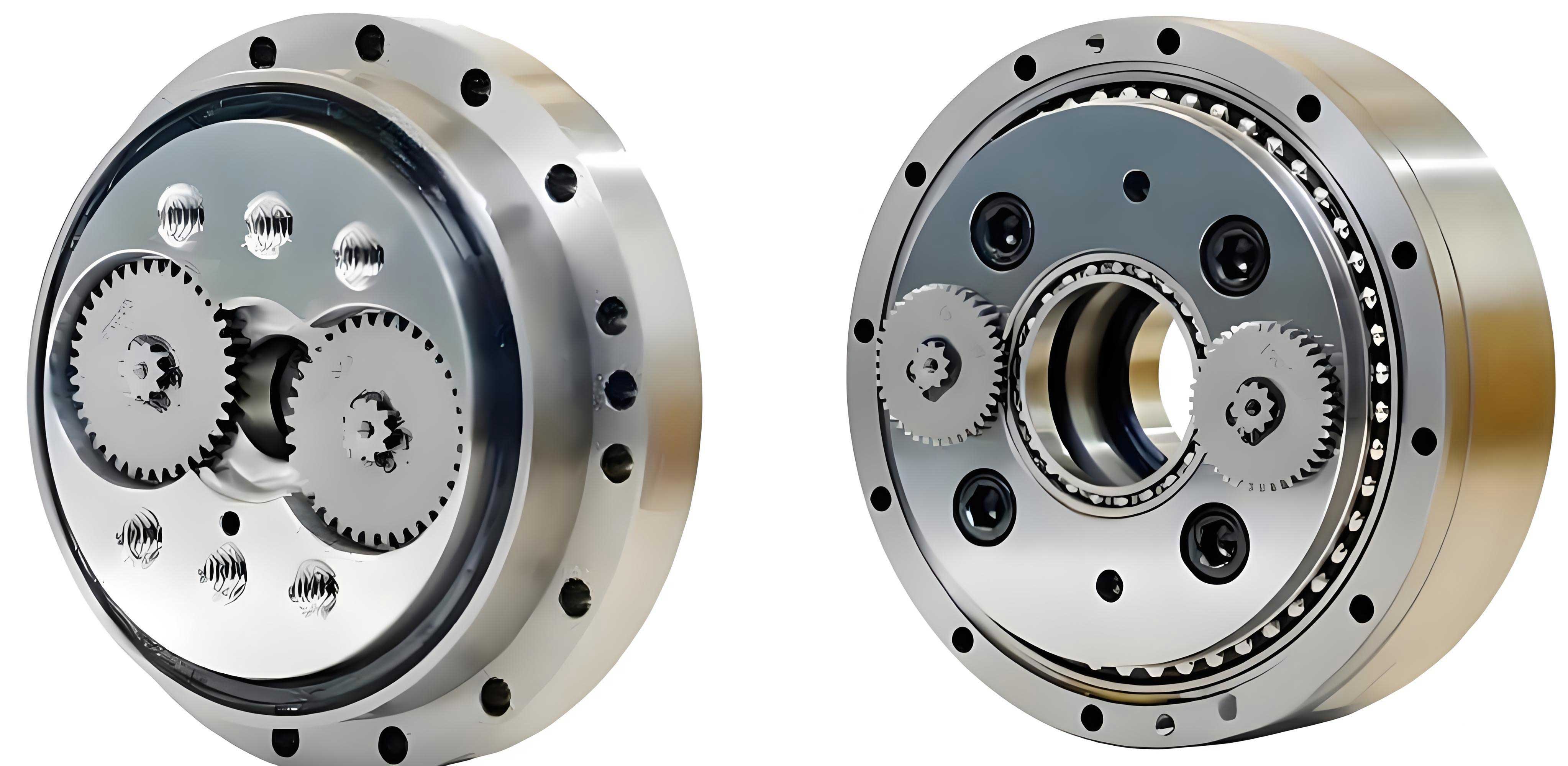
The overall lifespan of a complex assembly like a rotary vector reducer is dictated by its weakest critical component under fatigue. Analysis and experimentation consistently identify the needle roller bearings on the crankshaft (also called cycloidal pins or eccentric shafts) as the primary life-limiting element in most rotary vector reducer designs. These bearings operate at the highest relative speed within the reducer, experience significant and dynamically varying loads from the cycloidal disc meshing, and often have challenging lubrication and heat dissipation conditions. Therefore, an accurate life calculation for the rotary vector reducer hinges on a precise fatigue life analysis of these crankshaft bearings.
A detailed quasi-static force analysis of the cycloidal drive stage is essential to determine the load on each crankshaft bearing. The force transmitted from the cycloidal disc to the crankshaft bearing is periodic with the revolution of the crankshaft. For a rotary vector reducer with $\lambda$ crankshafts, the force $F$ on an individual bearing at an angular position $\theta$ can be derived as a function of the output torque $T$ and the reducer’s geometric parameters:
$$ F(\theta) = \frac{T}{2\lambda e Z_c r_0} \cdot \sqrt{(e Z_c)^2 + (1 + k_y^2) r_0^2 + 2 e Z_c r_0 (\cos \theta – k_y \sin \theta)} $$
where:
- $e$: Eccentricity
- $Z_c$: Number of teeth on the cycloidal disc
- $r_0$: Distribution circle radius of the crankshafts
- $k_y$: A dimensionless factor relating tangential and radial force components from the ring gear pins, typically defined as $k_y = \frac{2}{\pi}\left(\frac{1}{k} + \frac{k^2-1}{2k^2} \ln\frac{1+k}{1-k}\right)$ with $k = \frac{e Z_p}{R_p}$ ($Z_p$ is the number of ring gear pins, $R_p$ is the pin circle radius).
This equation shows that the load on the crankshaft bearing in a rotary vector reducer varies sinusoidally with the rotation angle $\theta$. For bearing life calculation, the mean equivalent dynamic load $F_m$ is required. For roller bearings, the ISO standard recommends using the $p=4$ norm (where $p$ is the life exponent, $10/3$ for roller bearings). Thus, the equivalent mean load is:
$$ F_m = \left( \frac{1}{2\pi} \int_0^{2\pi} F(\theta)^4 \, d\theta \right)^{1/4} $$
Substituting the expression for $F(\theta)$ and integrating reveals a simple proportionality between the equivalent mean bearing load $F_m$ and the output torque $T$:
$$ F_m = K \cdot T $$
where the constant $K$ is solely determined by the geometric parameters of the rotary vector reducer:
$$ K = \frac{ \sqrt[4]{ (eZ_c)^4 + 4(1+k_y^2)(eZ_c)^2 r_0^2 + (1+k_y^2)^2 r_0^4 } }{ 2\lambda e Z_c r_0 } $$
For a specific rotary vector reducer model, once the parameters are known, $K$ is a fixed value. For example, for a common RV-80E type reducer, the relationship is as shown in the following table, with the rated condition highlighted:
| Output Torque, $T$ (Nm) | Equivalent Mean Bearing Load, $F_m$ (N) |
|---|---|
| 500 | 2790 |
| 600 | 3348 |
| 700 | 3906 |
| 784 (Rated) | 4374 |
| 900 | 5022 |
| 1000 | 5580 |
The basic rating life $L_{10}$ of a rolling bearing, in hours, under constant load and speed is given by the standard ISO formula:
$$ L_{10} = \frac{10^6}{60 n’} \left( \frac{C_d}{F_m} \right)^{p} $$
where:
- $n’$: Rotational speed of the bearing (rpm). For a rotary vector reducer, $n’ = Z_p \cdot n_{\text{out}}$, where $n_{\text{out}}$ is the output rotational speed.
- $C_d$: Basic dynamic load rating of the bearing (N).
- $p$: Life exponent (10/3 for roller bearings).
Substituting $F_m = K T$, we obtain the rated life $L_0$ of the rotary vector reducer at its rated torque $T_0$ and rated output speed $n_0$:
$$ L_0 = \frac{10^6}{60 Z_p n_0} \left( \frac{C_d}{K T_0} \right)^{10/3} $$
This formula provides the theoretical lifespan under constant, rated operating conditions, a key reference point for the rotary vector reducer.
Real-world applications for industrial robots involve complex duty cycles with varying torque and speed. To calculate the service life under such variable conditions, we apply the Palmgren-Miner rule using the torque-life relationship. The damage per cycle at torque $T_i$ is proportional to $(T_i / T_0)^{10/3}$. The equivalent mean torque $T_m$ for the entire duty cycle, which would cause the same total damage, is derived as:
$$ T_m = \left( \frac{\sum (t_i n_i T_i^{10/3})}{\sum (t_i n_i)} \right)^{3/10} $$
where $t_i$ and $n_i$ are the time duration and output speed at torque level $T_i$ in the cycle. The equivalent mean speed $n_m$ is:
$$ n_m = \frac{\sum (t_i n_i)}{\sum t_i} $$
The total service life $L$ of the rotary vector reducer under this variable load profile is then:
$$ L = \frac{L_0 \cdot n_0 \cdot T_0^{10/3}}{n_m \cdot T_m^{10/3}} = \frac{10^5 \cdot C_d^{10/3}}{6 Z_p \cdot n_m \cdot (K T_m)^{10/3}} $$
This is the core mathematical expression for predicting the lifespan of a rotary vector reducer based on its specific duty cycle and fundamental fatigue strength principles.
Verifying these life calculations through physical testing under normal operating conditions is impractical due to the long duration involved. Accelerated life testing (ALT) is therefore essential. The most effective and controllable accelerating stress for a rotary vector reducer is mechanical load (torque), as its influence on bearing life is exponential (power of 10/3), compared to the linear influence of speed. An accelerated test applies a higher constant torque $T_a$ and possibly a higher speed $n_a$ to induce failure in a fraction of the time. The acceleration factor $A$, comparing the accelerated life $L_a$ to the rated life $L_0$, is:
$$ A = \frac{L_0}{L_a} = \frac{n_a}{n_0} \left( \frac{T_a}{T_0} \right)^{10/3} $$
To design a valid and representative ALT, the test should mimic the dynamic conditions of actual robot operation, such as frequent starts, stops, and reversals. A common test profile involves the rotary vector reducer driving a pendulum-like inertia load through a reciprocating swing motion (e.g., 180° back-and-forth). The output torque during such a swing has two main components: inertial torque ($J \epsilon$) due to angular acceleration/deceleration, and gravitational torque from the offset mass.
To realistically simulate robot motion profiles and minimize shock loads, an S-curve acceleration/deceleration control algorithm is implemented. This algorithm smoothly ramps the angular jerk (rate of change of acceleration), creating a seven-phase motion profile for each half-swing: jerk-up (increasing acceleration), constant acceleration, jerk-down (decreasing acceleration), constant velocity, jerk-up (increasing deceleration), constant deceleration, and jerk-down (decreasing deceleration to stop). The key kinematic parameters for a sample swing cycle are summarized below:
| Motion Phase | Duration, $\Delta t$ (s) | Angular Speed Change, $\Delta \omega$ (rad/s) | Angular Displacement, $\Delta \phi$ (rad) | Typical Angular Acceleration, $\epsilon$ (rad/s²) |
|---|---|---|---|---|
| Acceleration | 0.3 | 0 → $\pi/2$ | $3\pi/40$ | $+5\pi/3$ (mean) |
| Constant Velocity | 1.7 | $\pi/2$ (constant) | $17\pi/20$ | 0 |
| Deceleration | 0.3 | $\pi/2$ → 0 | $3\pi/40$ | $-5\pi/3$ (mean) |
| Dwell / Reverse | 1.0 | 0 | 0 | 0 |
The total output torque $T$ at any point is $T = J \epsilon + \sum (m_{a,i} g l_i \cos \phi_i)$, where $J$ is the load inertia, $g$ is gravity, and $m_{a,i}$, $l_i$, $\phi_i$ define the gravitational load. The maximum torque typically occurs during the initial part of the deceleration phase, where the inertial torque from negative acceleration adds to the gravitational torque. For an accelerated test targeting a maximum torque $T_a = 2.5 T_0$, the equivalent mean torque $T_m$ for the swing cycle can be calculated. Using the formulas above, the theoretical accelerated life $L_a$ and the acceleration factor $A$ can be predicted.
A test rig is constructed to execute this protocol. It consists of a servo motor driving the rotary vector reducer under test, whose output shaft is connected to a calibrated inertia arm with adjustable masses. A high-resolution absolute encoder or laser displacement sensor is used to continuously monitor the output angular position to track the degradation of positional repeatability—a key performance indicator for a failing rotary vector reducer. Temperature sensors monitor housing temperature, and vibration sensors may be used for ancillary data.
In a typical test on an RV-80E type rotary vector reducer with a theoretical rated life $L_0 \approx 6000$ hours under rated conditions, an accelerated test was run with $T_a = 2.5T_0$ and $n_a = n_0$. The theoretical acceleration factor and predicted accelerated life were:
$$ A_{\text{theory}} = \left( \frac{2.5 T_0}{T_0} \right)^{10/3} = (2.5)^{10/3} \approx 20.7 $$
$$ L_{a,\text{predicted}} = \frac{L_0}{A} = \frac{6000}{20.7} \approx 290.6 \text{ hours} $$
The test was run until a clear failure mode emerged. The primary data collected was the repeatability error of the end-of-swing position. Analysis of this data showed three distinct phases:
- Run-in Period (0-20 hours): A slight shift in positioning as internal stresses relaxed and components settled.
- Stable Operation (20-300 hours): Excellent and consistent repeatability with minimal variation.
- Degradation and Failure (300+ hours): A marked increase in positional scatter and drift, indicating loss of precision due to internal wear or fatigue damage.
The accelerated life $L_{a,\text{test}}$ was defined as the point at which the repeatability error exceeded a pre-defined functional threshold, which occurred at approximately 310 hours. Post-test teardown inspection confirmed spalling fatigue on the needle rollers of the crankshaft bearings, validating them as the life-limiting component.
The correlation between prediction and experiment is strong:
$$ \text{Relative Error} = \frac{|L_{a,\text{test}} – L_{a,\text{predicted}}|}{L_{a,\text{predicted}}} \times 100\% = \frac{|310 – 290.6|}{290.6} \times 100\% \approx 6.6\% $$
Furthermore, the achieved acceleration factor was $A_{\text{test}} = 6000 / 310 \approx 19.4$, very close to the theoretical value of 20.7. This close agreement validates the accuracy of the fatigue strength-based life calculation model for the rotary vector reducer. The S-curve motion profile successfully replicated realistic dynamic loading while enabling a test duration reduction from thousands of hours to just hundreds, demonstrating a highly effective and efficient accelerated life testing methodology for rotary vector reducers.