
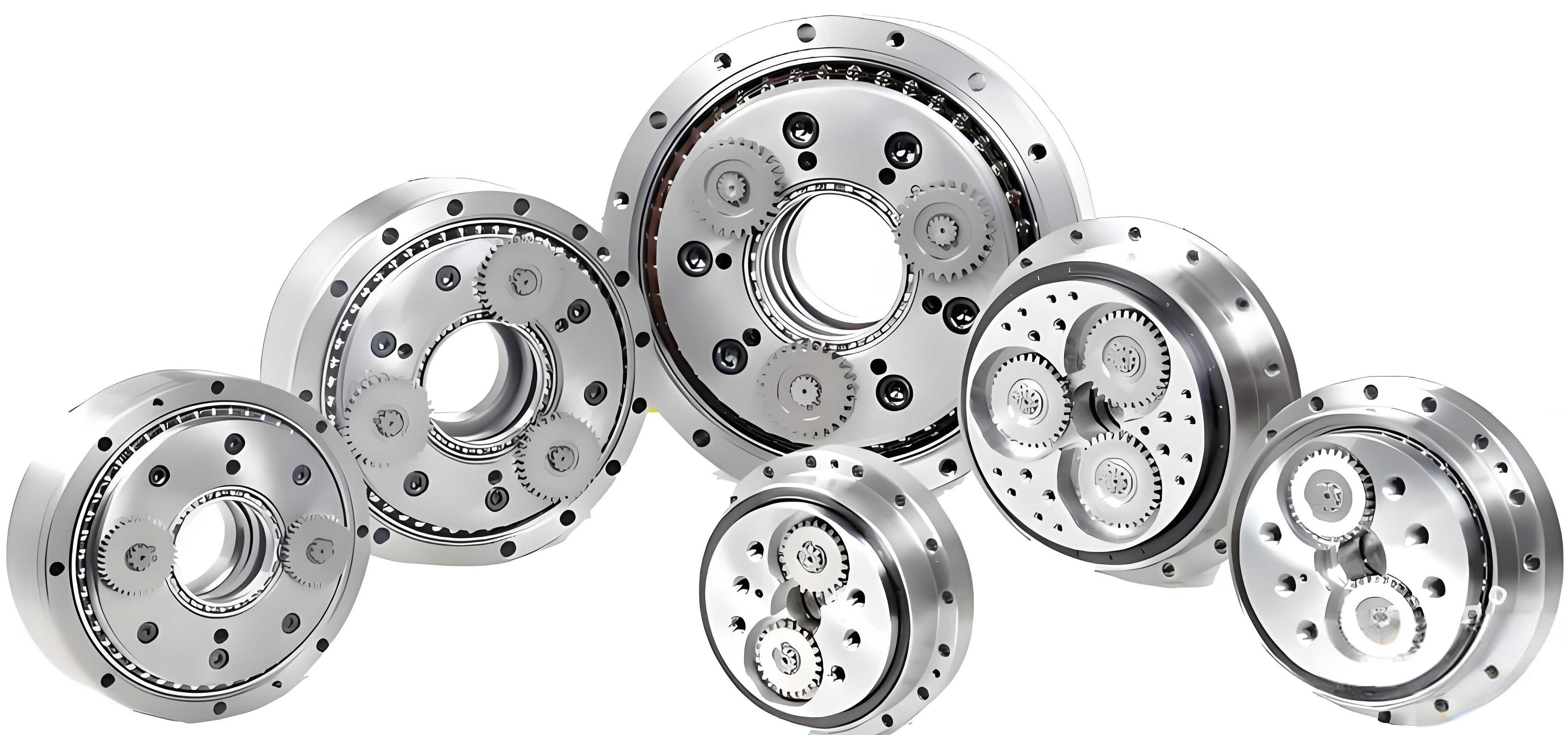
In the field of industrial robotics, joint actuators demand high precision, high transmission ratios, and exceptional stiffness. The rotary vector reducer, often abbreviated as RV reducer, has emerged as a critical component due to its ability to meet these stringent requirements. Its unique design, featuring a cycloidal gear and pin wheel mechanism, enables compact size, high torque capacity, and low backlash. However, the manufacturing of the cycloidal gear’s tooth profile is notoriously challenging, requiring precise control over the tooth form to ensure optimal meshing with the pin wheel. This article, from my perspective as a researcher in mechanical engineering, delves into the optimization of tooth profile modification for rotary vector reducers. I will explore conventional modification methods, introduce a novel segmentation-based modification approach, and validate it through a detailed case study. The goal is to present a method that not only enhances performance but also facilitates high-precision machining in industrial settings.
The rotary vector reducer operates on a two-stage reduction principle: a first stage involving a planetary gear train and a second stage utilizing a cycloidal drive. The heart of the RV reducer is the cycloidal disk, which meshes with a ring of pins. The tooth profile of this cycloidal disk is not a simple curve; it is derived from the epicycloidal or hypocycloidal family, depending on the design. To ensure smooth operation, minimize wear, and accommodate lubrication and manufacturing tolerances, the theoretical tooth profile must be modified. This process, known as tooth profile modification, aims to create a small clearance in non-working regions while maintaining conjugate meshing in the working region. Failure to properly modify the profile can lead to increased noise, vibration, and reduced lifespan of the rotary vector reducer.
Traditional modification methods for rotary vector reducers often rely on a combined approach, typically involving equal-distance and shift-distance modifications. This method, while effective, treats the entire tooth profile uniformly and often keeps specific modification amounts as proprietary industrial secrets. Let me break down the underlying principles. The standard tooth profile coordinates for a cycloidal gear are given by a set of parametric equations based on the generating circle rolling around the base circle. When considering modification, two primary parameters are introduced: the equal-distance modification amount, denoted as $\Delta r_{rp}$, which alters the radius of the roller pins virtually, and the shift-distance modification amount, $\Delta r_p$, which modifies the radius of the pin wheel’s pitch circle. The combined effect aims to introduce a controlled radial clearance $\Delta j$.
The mathematical formulation begins with the standard coordinates. Let $a$ be the eccentricity, $r_p$ the radius of the pin wheel pitch circle, $r_{rp}$ the radius of the roller pins, $Z_b$ the number of teeth on the cycloidal gear, and $Z_a$ the number of pins (where typically $Z_a = Z_b + 1$ for a standard RV design). The transmission ratio $i_H$ is $Z_b / Z_a$. The short-width coefficient $k_1$ is a crucial parameter defined as $k_1 = a Z_b / r_p$. The unmodified tooth profile coordinates $(x_c, y_c)$ as a function of the rolling angle $\phi’$ are:
$$ x_c = \left[ r_p – r_{rp} S^{1/2} \right] \cos\left( (1 – i_H) \phi’ \right) – \frac{a r_p}{r_p – Z_b r_{rp}} S^{1/2} \cos\left( i_H \phi’ \right) $$
$$ y_c = \left[ r_p – r_{rp} S^{1/2} \right] \sin\left( (1 – i_H) \phi’ \right) + \frac{a r_p}{r_p – Z_b r_{rp}} S^{1/2} \sin\left( i_H \phi’ \right) $$
where $S = 1 + k_1^2 – 2 k_1 \cos(\phi’)$. For the combined equal-shift modification, the modified coordinates $(x_c’, y_c’)$ become:
$$ x_c’ = \left[ r_p + \Delta r_p – (r_{rp} + \Delta r_{rp}) S_r^{1/2} \right] \cos\left( (1 – i_H) \phi’ \right) – \frac{a}{r_p + \Delta r_p} \left[ r_p + \Delta r_p – Z_b (r_{rp} + \Delta r_{rp}) S_r^{1/2} \right] \cos\left( i_H \phi’ \right) $$
$$ y_c’ = \left[ r_p + \Delta r_p – (r_{rp} + \Delta r_{rp}) S_r^{1/2} \right] \sin\left( (1 – i_H) \phi’ \right) + \frac{a}{r_p + \Delta r_p} \left[ r_p + \Delta r_p – Z_b (r_{rp} + \Delta r_{rp}) S_r^{1/2} \right] \sin\left( i_H \phi’ \right) $$
Here, $S_r^{1/2} = \sqrt{1 + k_1’^2 – 2 k_1′ \cos(\phi’)}$ and the modified short-width coefficient is $k_1′ = a Z_b / (r_p + \Delta r_p)$. The selection of $\Delta r_{rp}$ and $\Delta r_p$ is critical and often based on empirical rules, considering factors like oil film thickness and required backlash. To illustrate, consider the parameters for a common rotary vector reducer model, RV-60N. The key specifications are summarized in the table below.
| Parameter | Symbol | Value |
|---|---|---|
| Number of Pin Teeth | $Z_p$ | 40 |
| Eccentricity (mm) | $a$ | 1.3 |
| Pin Wheel Pitch Radius (mm) | $r_p$ | 136.9798 |
| Roller Pin Radius (mm) | $r_{rp}$ | 5.99 |
| Equal-Distance Modification (mm) | $\Delta r_{rp}$ | 0.036 |
| Shift-Distance Modification (mm) | $\Delta r_p$ | -0.026 |
Applying these modification values, the tooth profile changes. The working region maintains a conjugate meshing condition with the pins, while the tooth root and tip regions develop a small, uniform clearance. This method has been widely adopted in the industry for rotary vector reducers. However, it has limitations. The modification amounts are global, and the transition between the working and non-working regions is not explicitly controlled, which might lead to stress concentrations if not carefully calibrated. Furthermore, with the advent of CNC grinding machines, there is a growing need for a modification method that directly provides precise coordinate points for the entire tooth profile, enabling more flexible and accurate manufacturing.
This need leads me to propose a novel segmentation-based modification method for rotary vector reducers. The core idea is to treat the tooth profile not as a single entity but as three distinct segments: the tooth root non-working region, the working region, and the tooth tip non-working region. This approach aligns perfectly with the physical meshing process of a rotary vector reducer. During operation, only a specific portion of the cycloidal tooth is in conjugate contact with the roller pins at any given time. By identifying this working region precisely, we can apply perfect conjugate theory there and then design the non-working regions with controlled clearances using smooth fitting curves.
The first step is to determine the exact angular range of the working region. This is achieved by analyzing the meshing phase angle for each tooth of the cycloidal gear. The meshing phase angle $\phi_i$ for the i-th tooth can be derived from the geometry of the rotary vector reducer. For a standard design, the working region typically spans from the initial contact tooth to the final contact tooth. Using the parameters for the RV-60N rotary vector reducer, the meshing phase angles can be calculated. The results often show that teeth in the middle of the arc of contact have nearly constant phase angles, while those at the entry and exit have varying angles. By plotting the meshing phase angle function, we can identify a stable plateau which defines the working range $[\phi_B, \phi_C]$. For the RV-60N, this range was found to be approximately $[0.051, 0.291]$ radians.
Once the working region is defined, the coordinates for this segment are given by the standard conjugate equations, ensuring perfect meshing. For the non-working regions—the tooth root (from point A to B) and the tooth tip (from point C to D)—we employ cubic spline curves. The cubic spline ensures smooth continuity (C² continuity) at the junctions with the working region, preventing stress-raising sharp corners. The general form of a cubic spline segment is:
$$ y = a x^3 + b x^2 + c x + d $$
The coefficients $a, b, c, d$ for each spline segment are determined by enforcing boundary conditions: the coordinates at the endpoints (A, B, C, D) and the first derivative (slope) at the junctions B and C. The slopes at B and C are obtained from the derivative of the working region curve at those points, ensuring a smooth transition. For the tooth root segment AB, we often set a boundary condition at point A (the deepest point of the tooth root) with a specified radial clearance $\Delta$. Similarly, for the tooth tip segment CD, point D is at the tooth tip circle radius minus a clearance. The following table summarizes the endpoint coordinates for a single tooth flank, assuming symmetry about the tooth centerline.
| Point | Description | X-coordinate | Y-coordinate |
|---|---|---|---|
| A | Tooth Root Bottom | 0 | $R_{ia} – \Delta$ |
| B | Start of Working Region | $x(\phi_B)$ | $y(\phi_B)$ |
| C | End of Working Region | $x(\phi_C)$ | $y(\phi_C)$ |
| D | Tooth Tip Top | $x(\phi_D = \pi / Z_C)$ | $R_{ea} – \Delta$ |
Here, $R_{ia}$ is the root circle radius, $R_{ea}$ is the tip circle radius, $Z_C$ is the number of cycloidal teeth, and $\Delta$ is a user-defined clearance for lubrication and tolerance. The slopes are calculated as:
$$ \left. \frac{dy}{dx} \right|_{\phi = \phi_B} = \frac{ \frac{dy(\phi)}{d\phi} }{ \frac{dx(\phi)}{d\phi} } \Bigg|_{\phi = \phi_B}, \quad \left. \frac{dy}{dx} \right|_{\phi = \phi_C} = \frac{ \frac{dy(\phi)}{d\phi} }{ \frac{dx(\phi)}{d\phi} } \Bigg|_{\phi = \phi_C} $$
For the tooth tip segment CD, we solve the following system of equations to find the spline coefficients:
$$ y_C = a x_C^3 + b x_C^2 + c x_C + d $$
$$ y_D = a x_D^3 + b x_D^2 + c x_D + d $$
$$ \left. \frac{dy}{dx} \right|_{C} = 3a x_C^2 + 2b x_C + c $$
$$ \left. \frac{dy}{dx} \right|_{D} = 3a x_D^2 + 2b x_D + c $$
A similar system is solved for the tooth root segment AB. After obtaining the coefficients, we have explicit equations for all three segments. The complete tooth profile for one flank is the union of these segments. Due to symmetry, the other flank of the tooth is obtained by mirroring across the tooth centerline. Finally, the entire cycloidal gear profile is generated by rotating this single-tooth profile around the center by increments of $2\pi / Z_C$.
Let’s apply this novel method to the RV-60N rotary vector reducer. Using the previously determined working region $[\phi_B, \phi_C] = [0.051, 0.291]$ rad, we calculate the endpoint coordinates and slopes. For the working region (BC), the coordinates are given by the standard conjugate equations, which for our segmentation model can be written in a simplified form as:
$$ x(\phi) = \frac{1}{\sqrt{S}} \left[ r_p \sin\phi – \frac{k_1}{Z_p} \sin(Z_p \phi) + r_{rp} \left( k_1 \sin(Z_p \phi) – \sin\phi \right) \right] $$
$$ y(\phi) = \frac{1}{\sqrt{S}} \left[ r_p \cos\phi – \frac{k_1}{Z_p} \cos(Z_p \phi) – r_{rp} \left( k_1 \cos(Z_p \phi) – \cos\phi \right) \right] $$
where $S = 1 + k_1^2 – 2k_1 \cos(Z_p \phi)$, $k_1 = a Z_b / r_p$, and $Z_p = Z_a$ is the number of pins (40). The derivatives $dx/d\phi$ and $dy/d\phi$ can be derived analytically for slope calculations. For the RV-60N parameters, the slopes at B and C were computed as approximately 0.2543 and 0.0123, respectively. For the tooth tip segment, the slope at D (where $\phi_D = \pi / 40$) was found to be -0.0125. Solving the spline equations, we obtain the explicit cubic equations for the non-working segments. For the tooth tip segment CD, with $t_2$ representing the x-coordinate in the local segment coordinate system, the fitted curve is:
$$ y_2 = -0.002456 \left( (-1)^m t_2 \right)^3 – 0.0231512 \left( (-1)^m t_2 \right)^2 + 2.235642 \left( (-1)^m t_2 \right) + 26.56562 $$
Here, $m$ is a sign coefficient that accounts for the symmetry: $m=1$ for $\phi$ from $0$ to $\pi$, and $m=-1$ for $\phi$ from $\pi$ to $2\pi$. The final global coordinates are obtained by converting from the local spline coordinate system back to the polar/global system using a rotation transformation based on the tooth index. Similarly, for the tooth root segment AB, a cubic spline is derived. The complete piecewise function for a single tooth flank can be summarized as:
$$ f(x_n, y_n) = \begin{cases}
\text{Segment AB (Tooth Root):} & x_1 = (-1)^m t_1, \quad y_1 = \text{cubic in } t_1 \\
\text{Segment BC (Working Region):} & x(\phi), y(\phi) \text{ as conjugate equations} \\
\text{Segment CD (Tooth Tip):} & x_2 = (-1)^m t_2, \quad y_2 = \text{cubic in } t_2
\end{cases} $$
with global coordinates calculated as $x_{global} = \sin(\varphi) \sqrt{x_n^2 + y_n^2}$, $y_{global} = \cos(\varphi) \sqrt{x_n^2 + y_n^2}$, where $\varphi$ is the position angle of the tooth. This method yields a complete tooth profile with a perfectly conjugate working region and smoothly blended non-working regions with predetermined clearances. The clearances in the root and tip are directly controlled by the parameter $\Delta$ in the endpoint definitions, offering great flexibility for design optimization. This is a significant advantage for the rotary vector reducer, as it allows engineers to tailor the clearance based on lubrication needs, thermal expansion, and load conditions without affecting the meshing quality in the working zone.
To further illustrate the benefits, let’s compare the tooth profiles generated by the traditional combined modification and the new segmentation method for the rotary vector reducer. While the traditional method produces a continuous modified curve, the segmentation method explicitly defines regions. The transition in the segmentation method is guaranteed to be smooth (C² continuous) due to the cubic spline interpolation, whereas the traditional method’s transition depends on the global modification amounts and might not be optimally smooth. Moreover, the segmentation method provides direct coordinate points for CNC programming, which is invaluable for modern manufacturing of high-precision rotary vector reducers. The ability to export these piecewise equations directly to machine tool controllers simplifies the grinding process and reduces errors associated with approximation.
The impact of this optimization extends beyond mere geometry. The performance of a rotary vector reducer is heavily influenced by the tooth contact pattern, stress distribution, and torsional stiffness. By ensuring perfect conjugate action in the working region, the new method minimizes transmission error, which is a primary source of vibration and noise in precision drives like the rotary vector reducer. The controlled clearances in non-working regions ensure adequate space for lubricant flow, reducing friction and wear. Furthermore, the explicit mathematical model allows for advanced finite element analysis (FEA) to predict stress concentrations more accurately. Engineers can now perform parametric studies by varying the clearance $\Delta$ or the spline coefficients to optimize for maximum load capacity or minimum weight, all critical for advanced applications of rotary vector reducers in robotics and aerospace.
In conclusion, the novel segmentation-based tooth profile modification method presented here offers a systematic and flexible approach for optimizing rotary vector reducer gears. By dividing the tooth flank into working and non-working regions and applying conjugate theory and cubic spline fitting respectively, we achieve a design that ensures high-performance meshing, controlled clearances, and manufacturability. This method addresses the limitations of traditional combined modification, especially in the era of digital manufacturing. The explicit coordinate equations facilitate direct CNC machining, potentially improving accuracy and reducing production costs for rotary vector reducers. Future work could involve dynamic analysis to validate the vibration characteristics, multi-objective optimization of the spline parameters for different operating conditions, and extension to other types of cycloidal drives. The rotary vector reducer, with its critical role in robotics, stands to benefit significantly from such precise and adaptable design methodologies, pushing the boundaries of precision motion control.