
The evolution of intelligent manufacturing is fundamentally tied to the precision and reliability of its core components. Among these, the rotary vector reducer stands as a critical and costly element within industrial robotic joints, responsible for torque amplification and speed reduction. Its health directly impacts robotic accuracy, operational stability, and overall system longevity. However, monitoring the condition of a rotary vector reducer presents a significant challenge: during typical robotic tasks involving acceleration, constant velocity, and deceleration phases, the input speed to the reducer is time-varying and often not directly measurable. This unknown and variable speed complicates traditional vibration-based fault diagnosis, which relies on knowledge of characteristic fault frequencies derived from rotational speed. This article presents a comprehensive methodology for diagnosing faults in rotary vector reducers under such unknown speed conditions by synergistically analyzing motor current and housing vibration signals.
The core challenge stems from the operational reality of industrial robots. Performing tasks like welding, assembly, or painting, a robot joint frequently undergoes complex motion profiles. Directly instrumenting the high-speed input shaft of the rotary vector reducer for precise tachometer readings is often impractical in deployed systems. Without an accurate, real-time measure of the input rotational frequency ($f_s$), calculating the fault characteristic frequencies for internal components like the sun gear, planetary gears, or cycloid gears becomes impossible. These frequencies are defined by the gear mesh kinematics and are multiples of the fundamental shaft speeds. Consequently, effective fault diagnosis must first solve the problem of speed estimation before proceeding to feature extraction and health assessment.
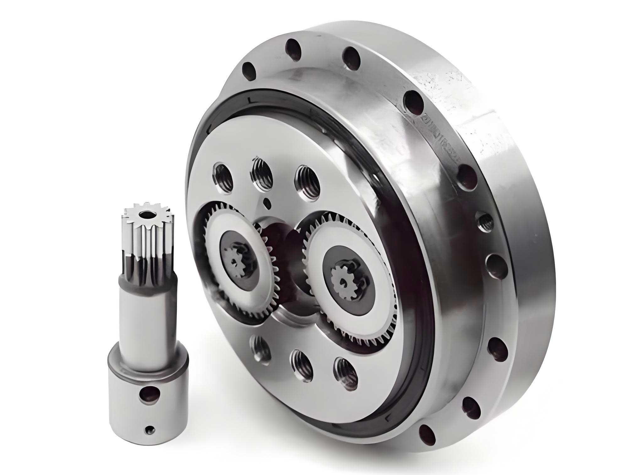
The proposed method employs a two-channel sensing approach. The three-phase current signals driving the joint’s servo motor are readily accessible from the motor drive cabinet. These current signals contain modulated information related to the motor’s rotational speed and load torque. Simultaneously, vibration acceleration signals are acquired from the housing of the rotary vector reducer, capturing the dynamic response of the internal gear train. The overall diagnostic workflow integrates signal processing, parameter-adaptive decomposition, and intelligent component selection, as conceptualized in the following sequence:
- Instantaneous Speed Estimation from Current: Analyze the motor current signal to estimate the time-varying instantaneous frequency, which corresponds to the motor’s electrical frequency. Convert this to the mechanical rotational frequency of the input shaft.
- Stationary Vibration Segment Extraction: Synchronously identify and extract segments of the vibration signal corresponding to periods of relatively constant estimated speed.
- Adaptive Signal Decomposition: Apply a parameter-optimized Variational Mode Decomposition (VMD) algorithm to the stationary vibration segment to break it down into intrinsic mode functions (IMFs).
- Fault-Sensitive IMF Selection: Utilize a multi-dimensional evaluation function to automatically identify the IMF(s) most laden with fault-related impulsive information.
- Envelope Analysis & Diagnosis: Perform envelope demodulation on the selected IMF(s) and analyze the resulting envelope spectrum against the calculated fault characteristic frequencies to diagnose the health state of the rotary vector reducer.
The advantage of this approach lies in its self-contained nature. It does not require external tachometers or pre-known motion profiles. It leverages commonly available electrical signals and standard vibration sensors to create a complete diagnostic picture for the rotary vector reducer, even amidst varying operational speeds.
Theoretical Foundations for Unknown-Speed Analysis
1. Instantaneous Frequency Estimation via Time-Frequency Analysis
Motor current signals in AC drives, particularly under loaded conditions, contain harmonic components whose frequencies are linked to the rotor speed. For a motor with $p$ pole pairs, the fundamental electrical frequency $f_m$ is related to the mechanical rotational speed $f_s$ (in Hz) by:
$$ f_s = \frac{f_m}{p} $$
During robot motion, $f_m$ varies with time. To track this variation, we treat the current signal as a non-stationary signal and employ high-resolution time-frequency analysis.
A powerful tool for this is the Linear Chirplet Transform (LCT), a generalization of the Short-Time Fourier Transform (STFT). The LCT introduces an additional chirp rate parameter $\alpha$ to rotate the analyzing basis in the time-frequency plane, providing superior concentration for signals with linear frequency modulations, which approximate the acceleration/deceleration phases of a robot joint. Given an analytic current signal $z(t)$ derived via the Hilbert Transform, the LCT is defined as:
$$ \text{TF}(t_0, \omega, \alpha, \sigma) = A(t_0) \int_{-\infty}^{+\infty} \bar{z}(t) \omega_\sigma(t-t_0) \exp(-j\omega t) dt $$
where $\bar{z}(t)$ is a rotated and shifted version of $z(t)$, $t_0$ is time, $\omega$ is angular frequency, $\sigma$ controls the width of the window function $\omega_\sigma$ (typically a Gaussian window), and $A(t_0)$ is a phase factor. The optimal $\alpha$ helps to “align” the transform with the signal’s frequency modulation, yielding a sharper time-frequency representation (TFR) $\text{TF}(t_0, \omega)$.
From the TFR, the instantaneous frequency (IF) ridge, $f_m(t)$, must be extracted. This is achieved through a path-finding algorithm that minimizes a cost function across time slices. Starting from an initial peak frequency at time $t_1$, the ridge at time $t_k$ is found by solving:
$$ f^*(t_k) = \min_{f(t_k)} \left\{ -|\text{TF}(t_k, f(t_k))|^2 + \lambda [f(t_k) – f^*(t_{k-1})]^2 \right\} $$
subject to $ f^*(t_{k-1}) – p_0 \leq f(t_k) \leq f^*(t_{k-1}) + p_1 $.
Here, $\lambda$ is a penalty parameter that controls the smoothness of the extracted ridge, and $p_0, p_1$ define the local search range. This adaptive ridge extraction robustly tracks the dominant electrical frequency $f_m(t)$ over time, from which the rotary vector reducer’s input shaft speed $f_s(t)$ is directly calculated.
2. Fault Characteristic Frequencies of the Rotary Vector Reducer
With the input speed $f_s$ known (or estimated), the characteristic fault frequencies for the two-stage rotary vector reducer can be determined. The reducer consists of a first-stage planetary gear train and a second-stage cycloid-pin gear mechanism. Let us define the component indices and parameters:
| Symbol | Component |
|---|---|
| 1 | Sun Gear |
| 2 | Planetary Gear |
| 3 | Front Carrier (Planetary Carrier) |
| 4 | Crank Shaft |
| 5 | Cycloid Gear |
| 6 | Pin Gear (Stationary) |
| 7 | Rear Carrier (Output Carrier) |
And the key parameters: $Z_1$ (sun gear teeth), $Z_2$ (planetary gear teeth), $Z_5$ (cycloid gear lobes), $Z_6$ (pin gear pins), $N_2$ (number of planetary gears). The transmission ratio $i$ of the rotary vector reducer is given by:
$$ i = \frac{Z_6}{Z_6 – Z_5} \cdot (1 + \frac{Z_2}{Z_1}) $$
The fundamental frequencies are calculated as follows, where $f_1 = f_s$ is the sun gear/shaft input frequency:
| Frequency Description | Formula |
|---|---|
| Planetary Gear Rotational Freq. | $f_2 = \frac{Z_1 Z_6}{(Z_5 – Z_6)(Z_1 + Z_2 Z_6)} f_1$ |
| Crank Shaft Rotational Freq. | $f_4 = f_2$ |
| Cycloid Gear Rotational Freq. | $f_5 = \frac{Z_1}{Z_1 + Z_2 Z_6} f_1$ |
| Planetary Carrier (Output) Freq. | $f_7 = \frac{Z_1}{Z_1 + Z_2 Z_6} f_1$ |
| 1st Stage Mesh Frequency | $f_{1c} = \frac{Z_1 Z_2 Z_6}{Z_1 + Z_2 Z_6} f_1$ |
| Sun Gear Fault Frequency (FTF) | $f_{1f} = \frac{f_{1c}}{Z_1 / N_2} = \frac{N_2 f_{1c}}{Z_1}$ |
| Planetary Gear Fault Frequency (FTF) | $f_{2f} = \frac{f_{1c}}{Z_2}$ |
These formulas provide the target frequencies for diagnostic analysis once $f_1$ is established from the current signal analysis.
3. Adaptive Vibration Decomposition with Parameter Optimization
Vibration signals from a faulty rotary vector reducer are typically nonlinear and non-stationary, containing modulated components from multiple sources. Variational Mode Decomposition (VMD) is a powerful technique to decompose such a signal $x(t)$ into $K$ discrete band-limited Intrinsic Mode Functions (IMFs) $u_k(t)$. It solves the following constrained variational problem:
$$ \min_{\{u_k\},\{\omega_k\}} \left\{ \sum_{k=1}^{K} \left\| \partial_t \left[ \left( \delta(t) + \frac{j}{\pi t} \right) * u_k(t) \right] e^{-j\omega_k t} \right\|_2^2 \right\} $$
subject to $$ \sum_{k=1}^{K} u_k = x(t) $$
where $\{u_k\} = \{u_1, …, u_K\}$ are the mode functions, $\{\omega_k\} = \{\omega_1, …, \omega_K\}$ are their center frequencies, and $\delta(t)$ is the Dirac delta. The solution is found via the Alternating Direction Method of Multipliers (ADMM).
The performance of VMD is highly sensitive to the selection of two parameters: the number of modes $K$ and the quadratic penalty factor $\alpha$ (balancing data fidelity and mode bandwidth). An inappropriate choice can lead to mode mixing or omission. To automate this selection, a Particle Swarm Optimization (PSO) algorithm is employed. The PSO searches for the parameter pair $(\alpha, K)$ that minimizes a fitness function defined as the minimum Envelope Entropy among all resulting IMFs. Envelope Entropy is a measure of sparsity and impulsiveness; a lower value often indicates a component with clearer periodic impulses, which is desirable for fault detection. The PSO updates particle positions and velocities as:
$$ \begin{bmatrix} \alpha^{id}_{new} \\ K^{id}_{new} \end{bmatrix} = \delta \cdot \begin{bmatrix} \alpha^{id} \\ K^{id} \end{bmatrix} + C_1 r_1 (p^{id}_{best} – \begin{bmatrix} \alpha^{id} \\ K^{id} \end{bmatrix}) + C_2 r_2 (g_{best} – \begin{bmatrix} \alpha^{id} \\ K^{id} \end{bmatrix}) $$
where $\delta$ is inertia, $C_1, C_2$ are acceleration coefficients, $r_1, r_2$ are random numbers, $p^{id}_{best}$ is the particle’s historical best, and $g_{best}$ is the global best. This optimization ensures the VMD is tailored to the specific vibration signal from the rotary vector reducer.
4. Multi-Dimensional Evaluation Function for IMF Selection
After decomposition, not all IMFs are equally useful for fault diagnosis. A robust method is needed to automatically select the IMF(s) most sensitive to the fault. This is achieved by constructing a Multi-Dimensional Evaluation Function (MDEF) based on three complementary metrics calculated for each IMF $u_i(t)$:
- Kurtosis (S): Measures the “peakiness” or impulsiveness of the signal in the time domain.
$$ S_i = \frac{E[(u_i – \mu_{u_i})^4]}{\sigma_{u_i}^4} $$
where $E[\cdot]$ is the expectation, $\mu$ is the mean, and $\sigma$ is the standard deviation. - Envelope Spectrum Kurtosis (V): Measures the impulsiveness in the frequency domain of the envelope signal $a_i(t)$ (obtained via Hilbert Transform: $a_i(t) = |Hilbert(u_i(t))|$).
$$ V_i = \frac{E[(a_i – \mu_{a_i})^4]}{\sigma_{a_i}^4} $$ - Envelope Entropy (E): Measures the uncertainty or randomness of the envelope signal’s energy distribution. A fault impulse train tends to have a lower, more ordered entropy.
$$ E_i = -\sum_{j=1}^{N} p_{i,j} \log(p_{i,j}), \quad \text{where} \quad p_{i,j} = \frac{a_i(j)}{\sum_{j=1}^{N} a_i(j)} $$
To combine these metrics into a single score, the Entropy Weight Method (EWM) is used. First, each metric is normalized. For Kurtosis and Envelope Spectrum Kurtosis (higher is better):
$$ S’_i = \frac{S_i – \min(S)}{\max(S) – \min(S)}, \quad V’_i = \frac{V_i – \min(V)}{\max(V) – \min(V)} $$
For Envelope Entropy (lower is better):
$$ E’_i = \frac{\max(E) – E_i}{\max(E) – \min(E)} $$
Next, the information entropy and then the weight for each metric across all $K$ IMFs are computed. For metric $S’$:
$$ s_i = \frac{S’_i}{\sum_{i=1}^{K} S’_i}, \quad e_S = -\frac{1}{\ln K} \sum_{i=1}^{K} s_i \ln(s_i), \quad w_S = \frac{1 – e_S}{(1-e_S)+(1-e_V)+(1-e_E)} $$
The weights $w_V$ and $w_E$ for $V’$ and $E’$ are computed similarly. The final Multi-Dimensional Evaluation score for the $i$-th IMF is:
$$ L_i = w_S \cdot S’_i + w_V \cdot V’_i + w_E \cdot E’_i $$
The IMF with the highest $L_i$ score is selected as the fault-sensitive component $u_l(t)$ for subsequent envelope analysis.
Experimental Validation and Case Study
The proposed methodology was validated using data from a rotary vector reducer test rig. The setup consisted of a servo motor driving an RV reducer, which in turn actuated a swing arm with an adjustable mass to simulate joint loading. The reducer’s motion was a reciprocating swing. Key components were instrumented: a triaxial accelerometer on the reducer housing, current sensors on the motor drive lines, and temperature sensors. Data was sampled at 6.25 kHz. Tests were conducted with different health states (healthy, sun gear pitting, planetary gear pitting) under various loads and swing speeds.
1. Instantaneous Speed Estimation Results
The three-phase motor current signal was analyzed. The Linear Chirplet Transform produced a high-concentration time-frequency representation. The adaptive ridge extraction algorithm successfully traced the dominant frequency component throughout the swing cycle. The result clearly showed the acceleration, constant-speed, and deceleration phases of the joint. During the constant-speed phase, the estimated electrical frequency $f_m$ was stable at approximately 151.4 Hz. With the motor’s pole pairs $p$ known, the input shaft speed to the rotary vector reducer was calculated as $f_s = f_m / p = 30.25$ Hz. This demonstrated the method’s capability to unobtrusively obtain the crucial speed information necessary for all subsequent fault frequency calculations.
2. Vibration Signal Analysis and Fault Diagnosis
Synchronized with the estimated speed, a 2-second segment of vertical vibration data from a constant-speed operational phase was extracted for a planetary gear pitting fault case. This stationary vibration signal was fed into the PSO-optimized VMD algorithm. The PSO convergence curve showed the algorithm effectively minimized the fitness function (minimum envelope entropy), settling on optimal parameters $(\alpha^*, K^*) = (4937, 9)$. The VMD with these parameters decomposed the signal into 9 IMFs.
The Multi-Dimensional Evaluation Function was then applied. The entropy weights for Kurtosis, Envelope Spectrum Kurtosis, and Envelope Entropy were calculated as 0.49, 0.27, and 0.23, respectively. The weighted scores $L_i$ for each IMF were computed. IMF #5 consistently achieved the highest score across multiple datasets, indicating it contained the most significant fault-related impulsive information. A visual comparison of the time-domain waveforms of IMF #5 and another low-scoring IMF (e.g., IMF #8) confirmed that IMF #5 exhibited much clearer periodic impact signatures.
The envelope spectrum was computed from the Hilbert Transform of the selected fault-sensitive component, IMF #5. The spectrum revealed distinct spectral lines at 10 Hz and its multiples (20 Hz, 30 Hz, etc.). Referring back to the fault frequency table calculated using the estimated $f_s=30.25$ Hz, the planetary gear fault frequency $f_{2f}$ was precisely 10 Hz. The strong presence of this frequency and its harmonics in the envelope spectrum provided conclusive evidence of a fault in the planetary gear stage of the rotary vector reducer. This end-to-end process validated the entire methodology for diagnosing faults under unknown, variable speed conditions.
Discussion and Comparative Analysis
The presented method addresses a significant practical gap in the condition monitoring of robotic systems. Traditional vibration analysis often assumes constant speed or requires a physical tachometer. Model-based approaches, while valuable, struggle with the complexity of accurately modeling the entire robot dynamics including the detailed nonlinearities of a rotary vector reducer. The data-driven, signal-processing-centric approach here offers a more direct and implementable solution.
The synergy between current and vibration signals is key. The current signal provides the “key” (rotational speed) to interpret the “code” (vibration spectrum) correctly. Without this key, the vibration signal from a variable-speed rotary vector reducer is largely uninterpretable for precise fault identification. The adaptive nature of the technique—from speed ridge extraction to VMD parameter optimization and IMF selection—makes it robust to changes in operational conditions and specific reducer parameters.
Comparative advantages of this integrated method can be summarized:
| Aspect | Proposed Integrated Method | Traditional Vibration-Only Methods | Model-Based Methods |
|---|---|---|---|
| Speed Requirement | Estimates speed internally from current; no tachometer needed. | Requires known constant speed or direct speed measurement. | May use estimated states from observers, but models are complex. |
| Handling Variable Speed | Explicitly designed for it; uses TFR and segments stationary data. | Generally performs poorly; suffers from spectral smearing. | Can be designed for it but requires accurate dynamic model. |
| Adaptability | High; parameters (VMD, IMF selection) are optimized from data. | Low; often relies on pre-set bandpass filters or fixed wavelet parameters. | Medium; model parameters may need updating with wear. |
| Implementation Cost | Low; uses existing motor current and standard accelerometers. | Medium; requires vibration sensors + potentially a tachometer. | High; requires extensive system identification and model development. |
| Fault Specificity | High; calculates exact fault frequencies from estimated speed. | Low under variable speed; cannot pinpoint exact fault frequency. | Potentially high, but dependent on model fidelity and fault incorporation. |
Conclusion and Future Perspectives
This article has detailed a robust and practical methodology for fault diagnosis in rotary vector reducers operating under unknown and time-varying speed conditions, typical of industrial robotic joints. The core innovation lies in the fusion of motor current signal analysis for instantaneous speed estimation and advanced vibration signal processing for fault feature extraction. The method successfully circumvents the need for direct speed measurement by deriving the input shaft frequency from current harmonics via high-resolution time-frequency analysis and ridge extraction. This estimated speed enables the accurate calculation of all component-specific fault characteristic frequencies for the complex gear train within the rotary vector reducer.
The vibration analysis pathway is equally adaptive. The use of Particle Swarm Optimization to tailor the Variational Mode Decomposition parameters ensures an effective separation of signal components without prior expert knowledge. The subsequent Multi-Dimensional Evaluation Function, incorporating Kurtosis, Envelope Spectrum Kurtosis, and Envelope Entropy weighted by their informational importance, provides an intelligent and automatic mechanism to isolate the fault-sensitive component from noise and other interferences. Final envelope demodulation of this component reveals clear spectral peaks at the predicted fault frequencies, enabling conclusive diagnosis.
Validation on an experimental rotary vector reducer test rig with seeded planetary gear faults confirmed the method’s effectiveness. It accurately identified the fault type under simulated robotic operating conditions involving speed variation. This approach enhances the feasibility of implementing condition-based maintenance for industrial robots without major hardware modifications, leveraging signals that are often already accessible within the control system.
Future work can extend this methodology in several directions. Firstly, the instantaneous frequency estimation could be further refined using more advanced multi-ridge extraction techniques to handle cases with strong load modulation or multiple harmonic interactions in the current signal. Secondly, the multi-dimensional evaluation function could be expanded or its weighting scheme could be learned through machine learning models trained on a broader set of fault data from various rotary vector reducer models and failure modes. Finally, integrating this diagnostic framework into an online or edge-computing system for real-time health assessment of robotic joints in production environments represents the ultimate practical goal, paving the way for truly predictive maintenance in smart factories.