
The pursuit of high precision, compact power transmission in demanding applications such as industrial robotics and aerospace has positioned the rotary vector reducer as a critical component. Its advantages of high torsional stiffness, compact design, and significant load-bearing capacity are well-documented. However, the operational reliability of these complex mechanical systems under harsh conditions remains a paramount concern, particularly during the design phase where failure data is scarce. This article explores a methodology for predicting the reliability of rotary vector reducer systems using logical fault models, leveraging handbook data from similar components to inform design decisions and identify potential weak links before physical prototyping.
The core principle of this predictive approach lies in constructing a logical model of the system’s failure behavior. A rotary vector reducer is decomposed into its functional subsystems and constituent components. The reliability relationship between these components—whether they are arranged in series, parallel, or a combination thereof—is defined based on their functional interdependence. For a series system, the failure of any single component causes the entire subsystem to fail. For parallel (redundant) arrangements, all components must fail for the subsystem to fail. The overall system reliability is then mathematically synthesized from these subsystem models.
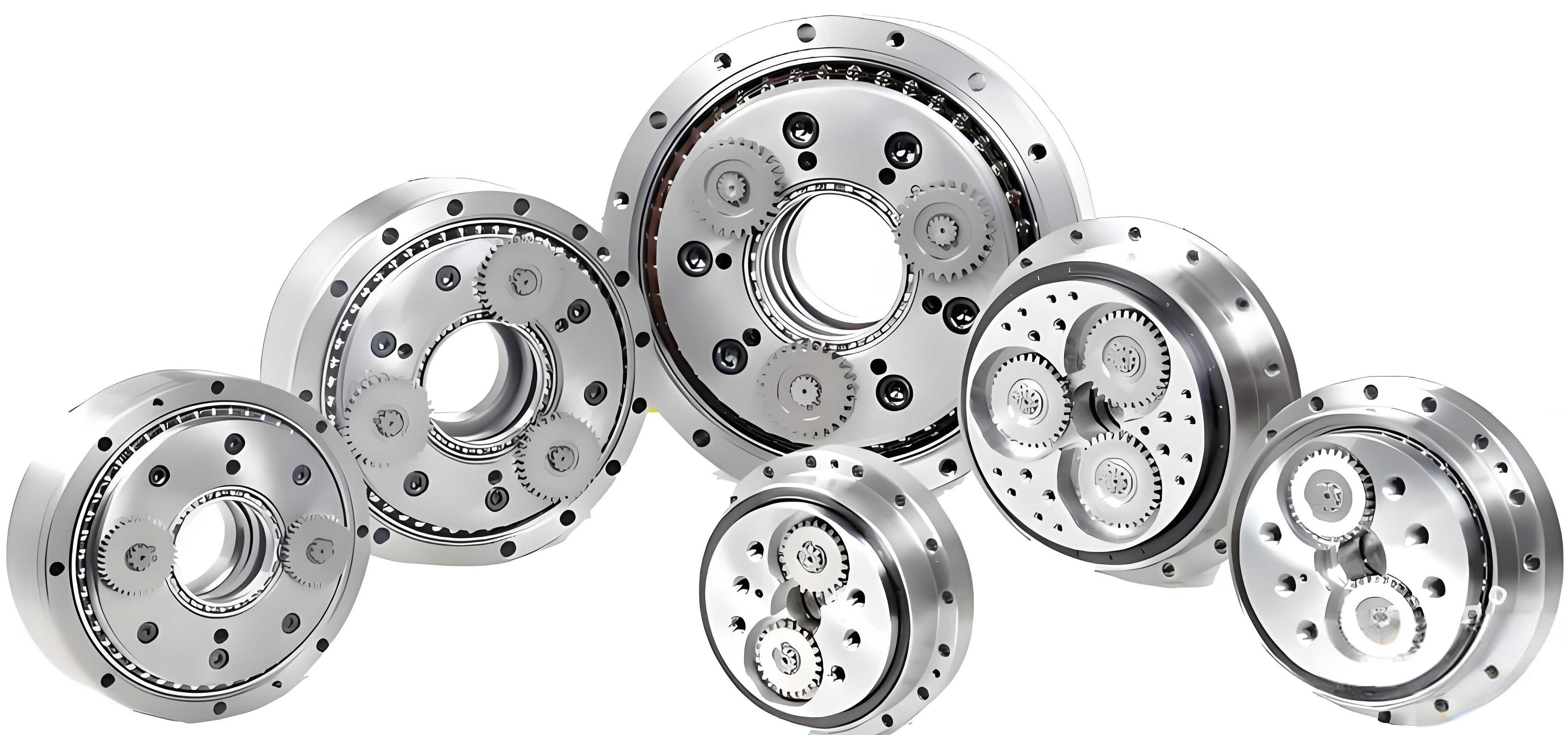
The transmission principle of a typical rotary vector reducer involves a two-stage process. The first stage is a planetary gear train, and the second is a cycloidal pin-wheel mechanism. This creates a closed differential system. The sun gear, connected to the input shaft, drives planetary gears. These planetary gears, fixed to crankshafts, induce an eccentric motion. Two cycloidal gears, mounted 180 degrees apart on these crankshafts, mesh with a ring of stationary needle pins. The resultant motion of the cycloidal gears—a combination of revolution and opposite-direction rotation—is output through a carrier mechanism. Predicting the reliability of such a system requires modeling both the planetary gear subsystem and the cycloidal gear subsystem independently before integrating them.
Reliability prediction is an iterative process that runs parallel to design evolution. It begins with a clear definition of the rotary vector reducer’s function, failure criteria, and expected operating conditions. A reliability block diagram (RBD) is then constructed, breaking down the system to its basic component level. A mathematical model is established based on the RBD’s logic. The reliability of each basic component is estimated, often using standardized handbooks like Non-electronic Parts Reliability Data (NPRD) which provide failure rate estimates for generic part types (e.g., “gear,” “deep groove ball bearing”) under various environmental and stress conditions. These component estimates are aggregated according to the system model to predict the reliability of subsystems and the entire rotary vector reducer. The results feed back into the design process, guiding reliability allocations and highlighting areas for improvement.
Mathematical Foundation for System Reliability Modeling
For a majority of mechanical systems like the rotary vector reducer, the system fails if any critical component fails. This functional relationship is accurately represented by a series reliability model. Let the lifetime of the i-th component be a random variable $X_i$. The reliability of that component at time $t$ is defined as the probability that its lifetime exceeds $t$:
$$
R_i(t) = P\\{X_i > t\\} \\quad (i = 1, 2, 3, \\ldots, n)
$$
Assuming statistical independence between component failures—a common simplifying assumption in early-stage analysis—the reliability of a series system with $n$ components is the product of their individual reliabilities:
$$
R_s(t) = \\prod_{i=1}^{n} R_i(t)
$$
If the failure rate function for each component is $\lambda_i(t)$, the component reliability is $R_i(t) = e^{-\int_0^t \lambda_i(u) du}$. Substituting this into the series system formula yields:
$$
R_s(t) = \\prod_{i=1}^{n} e^{-\int_0^t \lambda_i(u) du} = e^{-\int_0^t \sum_{i=1}^{n} \lambda_i(u) du} = e^{-\int_0^t \lambda_s(u) du}
$$
This shows that the system failure rate $\lambda_s(t)$ for a series system is the sum of the individual component failure rates:
$$
\lambda_s(t) = \\sum_{i=1}^{n} \lambda_i(t)
$$
A critical reliability metric is the Mean Time Between Failures (MTBF), calculated as the integral of the system reliability function over all time:
$$
\\text{MTBF} = \\int_0^{\infty} R_s(t) dt = \\int_0^{\infty} e^{-\int_0^t \lambda_s(u) du} dt
$$
A widely used simplification, especially when precise life data is unavailable, is to assume components have a constant failure rate, implying their lifetimes follow an exponential distribution. In this case, $\lambda_i(t) = \lambda_i$ (a constant). The system failure rate becomes a constant sum, and the MTBF simplifies to its reciprocal:
$$
\\lambda_s = \\sum_{i=1}^{n} \lambda_i, \\quad \\quad \\text{MTBF} = \\frac{1}{\lambda_s}
$$
For subsystems with redundancy (parallel arrangements), the reliability calculation differs. For a simple parallel system of $m$ identical components where all must fail to cause subsystem failure, the subsystem reliability $R_p(t)$ is:
$$
R_p(t) = 1 – \\prod_{j=1}^{m} (1 – R_j(t)) = 1 – (1 – R_c(t))^m
$$
where $R_c(t)$ is the reliability of a single component within the parallel set. In a complex system like a rotary vector reducer, subsystems often contain mixtures of series and parallel elements, requiring a stepwise calculation combining both formulas.
Case Study: Reliability Prediction for Key Subsystems of a Rotary Vector Reducer
1. Planetary Gear Subsystem (Series System Analysis)
The planetary gear stage of a rotary vector reducer can be effectively modeled as a series system. Its basic reliability block diagram includes the input shaft, sun gear, multiple planetary gears, their supporting bearings, crankshafts, and retaining elements. Failure of any of these items can halt the transmission of motion. Using the component count method and consulting failure rate databases for similar mechanical parts under comparable load and environmental conditions, we can populate a failure rate table.
| Component Name | Component Type | Quantity (q) | Failure Rate Estimate ($\lambda_i$, $\\times 10^{-6}$/h) | Aggregate Failure Rate ($q \\times \lambda_i$) |
|---|---|---|---|---|
| Sun Gear | Mechanical Gear | 1 | 1.00 | 1.00 |
| Planetary Gear | Mechanical Gear | 2 | 0.245 | 0.49 |
| Support Bearing | Deep Groove Ball Bearing | 2 | 58.00 | 116.00 |
| Crankshaft Segment | Machined Shaft | 2 | 3.383 | 6.766 |
| Retaining Ring | Fastener | 2 | 1.052 | 2.104 |
The system failure rate $\lambda_{s\_planetary}$ is the sum of the aggregate failure rates:
$$
\lambda_{s\\_planetary} = \\sum (q \\cdot \\lambda_i) = 1.00 + 0.49 + 116.00 + 6.766 + 2.104 = 126.36 \\times 10^{-6} / \\text{h}
$$
Assuming constant failure rates (exponential distribution), the MTBF and reliability at mission time $t=1000$ hours are:
$$
\\text{MTBF}_{planetary} = \\frac{1}{\\lambda_{s\\_planetary}} \\approx 7,915 \\ \\text{hours}
$$
$$
R_{planetary}(1000) = e^{-\\lambda_{s\\_planetary} \\cdot t} = e^{-126.36 \\times 10^{-6} \\times 1000} \\approx 0.8812
$$
A reliability function plot over time, $R(t)=e^{-126.36 \\times 10^{-6} t}$, reveals a steep decline. Analysis of the contribution matrix shows that support bearings constitute approximately $\frac{116.00}{126.36} \\approx 91.8\\%$ of the total subsystem failure rate. This unequivocally identifies them as the critical reliability bottleneck. Enhancing the planetary stage’s reliability, therefore, hinges on selecting bearings with a significantly lower failure rate, possibly through higher precision grades, superior materials, or modified lubrication strategies.
2. Cycloidal Pin-Wheel Subsystem (Mixed Series-Parallel System Analysis)
The cycloidal drive stage presents a more complex reliability logic. While the overall subsystem is in series with the planetary stage, it contains internal redundancies. For instance, two cycloidal gears share the load, and multiple needle pins form a load-sharing ring. A task reliability block diagram must reflect this. Key elements include the parallel paths of the two cycloidal gears, the crankshaft bearings, the set of needle pins (modeled as a $k$-out-of-$n$ system, but often simplified as a series string for conservatism), and the output mechanism with its pins and sleeves.
| Component Group | Code | Quantity | Failure Rate Estimate ($\lambda_i$, $\\times 10^{-6}$/h) | Reliability Logic |
|---|---|---|---|---|
| Cycloidal Gear | A | 2 | 15.40 | Parallel (Active Redundancy) |
| Bearing (Crankshaft) | B | 2 | 82.60 | Series (Critical Support) |
| Needle Pin Assembly | C | 40 | 5.78 | Series (Conservatively) |
| Needle Bearing (Roller) | D | 4 | 78.564 | Series |
| Output Pin & Sleeve | E | 8 (4 pairs) | 2.54 (Pin), 5.00 (Sleeve) | Series per station, Parallel across stations* |
*Complex logic simplified here for calculation; output pins are often in a parallel-series configuration.
The reliability calculation for the cycloidal gear stage at $t=1000$ hours proceeds stepwise:
Step 1: Parallel Cycloidal Gears. $R_A = e^{-15.40 \times 10^{-6} \times 1000} \approx 0.9847$. For two in parallel: $R_{A\_parallel} = 1 – (1 – R_A)^2 \approx 0.9998$.
Step 2: Crankshaft Bearings (Series). $R_B = e^{-82.60 \times 10^{-6} \times 1000} \approx 0.9207$. For two: $R_{B\_series} = (R_B)^2 \approx 0.8477$.
Step 3: Needle Pin Ring (40 in series, conservative). $R_C = e^{-5.78 \times 10^{-6} \times 1000} \approx 0.9942$. For 40: $R_{C\_series} = (R_C)^{40} \approx 0.7913$.
Step 4: Needle Roller Bearings (4 in series). $R_D = e^{-78.564 \times 10^{-6} \times 1000} \approx 0.9244$. For four: $R_{D\_series} = (R_D)^4 \approx 0.7301$.
Step 5: Simplified Output Stage. Assuming a critical series path for a representative pin/sleeve pair: $R_{E\_single} = e^{-(2.54+5.00)\times 10^{-6} \times 1000} \approx 0.9925$.
Combining these major series elements gives an estimated subsystem reliability:
$$
R_{cycloidal}(1000) \\approx R_{A\\_parallel} \\times R_{B\\_series} \\times R_{C\\_series} \\times R_{D\\_series} \\times R_{E\\_single}
$$
$$
R_{cycloidal}(1000) \\approx 0.9998 \\times 0.8477 \\times 0.7913 \\times 0.7301 \\times 0.9925 \\approx 0.388
$$
This simplified calculation, particularly the conservative treatment of the needle pin ring as a pure series system, yields a very low reliability figure, highlighting the sensitivity of the model to the assumed failure logic of highly redundant components. A more accurate model for the pin ring would use a load-sharing $k$-out-of-$n$:G model, which would yield a significantly higher reliability. Nevertheless, the analysis clearly shows that the bearings (both crankshaft and needle roller types) and the cycloidal gears themselves are major contributors to the failure rate. The combined failure rate contribution from bearings in this subsystem can exceed 75%, confirming them again as the primary target for reliability enhancement in the rotary vector reducer design.
Sensitivity Analysis and Design Improvement Strategies
The predictive model allows for quantitative sensitivity analysis. By varying the failure rate of a specific component in the model, we can observe the impact on the overall system MTBF or mission reliability. For instance, if the bearing technology is improved, reducing its failure rate by 50%, the system-level improvement can be calculated. Let $\Delta \lambda_{bearing}$ be the reduction in aggregate bearing failure rate. The new system failure rate is $\lambda_s’ = \lambda_s – \Delta \lambda_{bearing}$. The improvement in MTBF is:
$$
\\Delta \\text{MTBF} = \\frac{1}{\\lambda_s’} – \\frac{1}{\\lambda_s}
$$
The relative improvement is more pronounced when the original bearing contribution is high. This quantifiable relationship provides a powerful cost-benefit tool for designers. Beyond component selection, the logical fault model for the rotary vector reducer also informs maintenance strategies. Components with high failure rates and series relationships are prime candidates for condition monitoring or scheduled replacement.
Conclusion and Future Directions
The methodology of using logical fault models, underpinned by handbook failure rate data and series-parallel reliability mathematics, provides a powerful and practical tool for predicting the reliability of complex mechanical systems like the rotary vector reducer during the design phase. It transforms qualitative design judgments into quantitative reliability estimates, enabling objective comparison of different design configurations. The case studies consistently identify rolling element bearings as the predominant reliability bottleneck in both the planetary and cycloidal stages of the rotary vector reducer. This insight directs engineering effort towards procuring higher-grade bearings, optimizing bearing mounting and preload, and ensuring impeccable lubrication as the most effective means of improving the predicted MTBF of the entire system.
Future advancements in this field will focus on increasing the accuracy of the predictions. This involves moving beyond the exponential distribution assumption to incorporate more representative lifetime distributions like the Weibull distribution, which can model wear-out failures prevalent in mechanical components. Furthermore, integrating physics-of-failure models that relate specific failure modes (e.g., pitting, wear) to material properties, loads, and lubrication conditions will allow for more nuanced predictions tailored to the specific design and duty cycle of the rotary vector reducer. The integration of logical fault modeling with real-time condition monitoring data will eventually pave the way for dynamic reliability prediction and proactive maintenance scheduling, ensuring the highest levels of operational availability for systems dependent on the precision of the rotary vector reducer.