
In modern industrial applications, particularly in robotics and precision machinery, the performance and longevity of transmission components are critical. Among these, the RV reducer stands out as a key element due to its high torque capacity, compact design, and superior accuracy. As demands for operational reliability and precision increase, understanding the degradation of accuracy life in RV reducers becomes paramount. Accuracy life refers to the duration over which the transmission accuracy, such as transmission error, remains within acceptable thresholds before degradation leads to failure. This metric is a vital design and operational criterion, reflecting the RV reducer’s ability to maintain performance under stress. In this article, I explore the degradation characteristics of RV reducers, focusing on modeling approaches and reliability assessment methods to enhance predictive maintenance and design optimization. The goal is to provide a comprehensive framework for evaluating accuracy life, leveraging stochastic degradation models and machine learning techniques to improve the reliability of RV reducers in real-world applications.
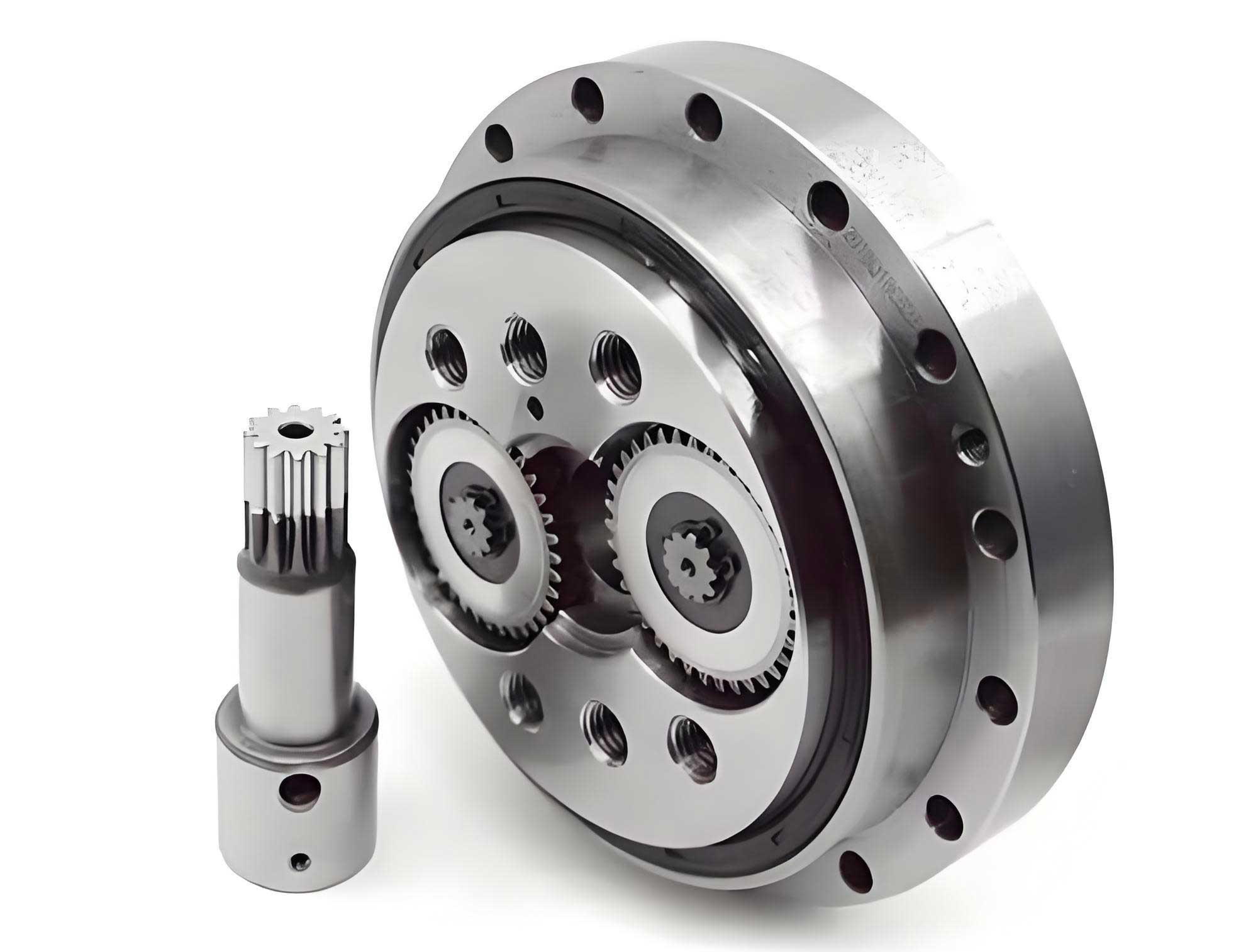
The RV reducer, a type of precision cycloidal drive, is widely used in industrial robots, aerospace systems, and engineering machinery. Its complex structure involves multiple gears and bearings, which are subject to wear and tear over time, leading to gradual degradation in transmission accuracy. This degradation manifests as increases in transmission error, which can affect the positional accuracy and repeatability of robotic systems. Therefore, monitoring and predicting the accuracy life of RV reducers is essential for ensuring system reliability and minimizing downtime. Traditional approaches to lifespan assessment often focus on fatigue life, but accuracy life has gained attention due to its direct impact on operational precision. I aim to address this by developing a methodology that combines degradation modeling with vibration-based prediction, offering a robust tool for reliability evaluation.
To achieve this, I propose a two-stage approach. First, I employ a Gamma process to model the stochastic degradation of transmission accuracy in RV reducers, capturing the monotonic increase in error over time. The Gamma process is suitable for such applications because it accounts for non-negative, independent increments, aligning with the gradual wear observed in mechanical systems. Second, I integrate a Gaussian process regression model, optimized using genetic algorithms, to predict transmission accuracy based on vibration signal features. This allows for real-time updates to the degradation model, enhancing the accuracy of reliability assessments. By combining these methods, I provide a dynamic framework for evaluating the accuracy life of RV reducers, with potential applications in predictive maintenance and design improvement. Throughout this article, I emphasize the importance of RV reducers in industrial contexts, and I repeatedly reference RV reducers to underscore their significance in precision transmission systems.
The foundation of this work lies in the concept of accuracy retention, which quantifies how well a mechanical system maintains its geometric accuracy under operational conditions. For RV reducers, key accuracy metrics include transmission error and backlash, with transmission error being a primary indicator of degradation. Transmission error is defined as the difference between the actual output rotation angle and the theoretical angle, normalized by the transmission ratio. Mathematically, for an RV reducer, the transmission error \(E\) can be expressed as:
$$E = \frac{\theta_{\text{in}}}{i_T} – \theta_{\text{out}}$$
where \(\theta_{\text{in}}\) is the actual input angle, \(\theta_{\text{out}}\) is the actual output angle, and \(i_T\) is the transmission ratio. The transmission accuracy \(\theta\) is then derived as the range of transmission error values over a cycle:
$$\theta = E_{m1} – E_{m2}$$
Here, \(E_{m1}\) and \(E_{m2}\) represent the maximum and minimum transmission error values, respectively. This metric serves as the degradation indicator for accuracy life in RV reducers, with failure thresholds typically defined based on industry standards. For instance, according to guidelines similar to GB/T 30819-2014, RV reducers are classified into accuracy grades, where a transmission accuracy exceeding 60 arcseconds may indicate failure for certain applications. Thus, tracking \(\theta\) over time allows for the assessment of accuracy life degradation in RV reducers.
To model this degradation, I adopt a Gamma process, a stochastic tool well-suited for monotonic degradation paths. The Gamma process is defined such that the degradation increment \(X(t)\) at time \(t\) follows a Gamma distribution with shape parameter \(\alpha(t)\) and scale parameter \(\beta\). The probability density function of \(X(t)\) is given by:
$$f_{X(t)}(x) = \frac{\beta^{\alpha(t)}}{\Gamma[\alpha(t)]} x^{\alpha(t)-1} e^{-\beta x} I_{(0,\infty)}(x)$$
where \(\Gamma[\cdot]\) is the Gamma function, and \(I_{(0,\infty)}(x)\) is an indicator function. The reliability function \(R(t)\), representing the probability that the degradation has not exceeded a failure threshold \(D_f\) by time \(t\), can be derived as:
$$R(t) = P(X(t) < D_f) = \frac{\Gamma[\alpha(t), D_f \beta]}{\Gamma[\alpha(t)]}$$
Here, \(\Gamma[\alpha(t), D_f \beta]\) is the incomplete Gamma function. This formulation provides a probabilistic framework for assessing the accuracy life of RV reducers, but it requires accurate estimation of parameters \(\alpha(t)\) and \(\beta\). I estimate these using historical degradation data from performance tests on RV reducers, applying methods such as the matrix approach and maximum likelihood estimation. For example, based on experimental data from an RV80E reducer, the estimated parameters might be \(\alpha = 2.72\) and \(\beta = 0.78\), as summarized in the table below:
| Degradation Indicator | Shape Parameter \(\alpha\) | Scale Parameter \(\beta\) |
|---|---|---|
| Transmission Error Increment | 2.72 | 0.78 |
However, relying solely on historical data may not capture real-time degradation changes in RV reducers. To address this, I incorporate vibration signal analysis, as vibration features often correlate with mechanical wear and can provide early indicators of accuracy loss. In experiments, I collect vibration data from RV reducers under constant stress conditions, using triaxial accelerometers mounted on the reducer housing. The vibration signals are sampled at 2 kHz over 180-second intervals, synchronized with transmission error measurements. From these signals, I extract features such as root mean square (RMS), variance, kurtosis, and time-frequency energy, which exhibit monotonic trends aligned with degradation in RV reducers. A subset of this feature data is shown in the table below, illustrating the variation over time for an RV reducer:
| Time (h) | RMS | Variance | Kurtosis Factor | Time-Frequency Energy |
|---|---|---|---|---|
| 500 | 1.5000 | 1.8449 | 7.2721 | 0.8974 |
| 500 | 1.3333 | 1.7910 | 8.5758 | 1.1145 |
| 1000 | 1.1806 | 1.3694 | 7.6425 | 0.8692 |
| 1500 | 0.9167 | 1.0762 | -0.7543 | 0.5547 |
| 2000 | -0.1250 | -0.2932 | -9.5952 | -0.2637 |
| 2500 | -1.9306 | -3.2753 | -15.0549 | -1.0526 |
| 3000 | -2.9583 | -6.4206 | -18.7732 | -0.8150 |
These features serve as inputs for a prediction model to estimate transmission accuracy in RV reducers. Among various regression techniques, I develop a Gaussian process regression (GPR) model optimized via genetic algorithms (GA), referred to as GA-GPR. Gaussian processes are advantageous for their ability to model uncertainty and non-linear relationships, making them ideal for degradation prediction in RV reducers. The GA optimization tunes hyperparameters such as the covariance function to improve predictive accuracy. The GPR model assumes that the observed data \(y\) is related to inputs \(x\) through a function \(f(x)\) plus noise \(\epsilon\):
$$y = f(x) + \epsilon, \quad \epsilon \sim N(0, \sigma_n^2)$$
The joint distribution of training outputs \(y\) and test predictions \(f_*\) is given by:
$$\begin{bmatrix} y \\ f_* \end{bmatrix} \sim N\left(0, \begin{bmatrix} C(X, X) + \sigma_n^2 I & C(X, X_*) \\ C(X_*, X) & C(X_*, X_*) \end{bmatrix}\right)$$
where \(C(\cdot, \cdot)\) is the covariance matrix, and \(X\) and \(X_*\) are training and test inputs, respectively. The posterior distribution for predictions is then:
$$f_* | X, Y, x_* \sim N(\mu(x_*), \text{var}(x_*))$$
To validate the GA-GPR model, I compare it with other regression approaches, such as backpropagation neural networks (BPNN) and particle swarm optimization-enhanced BPNN (PSO-BPNN), using metrics like root mean square error (RMSE), relative error (RE), coefficient of determination (\(R^2\)), and computation time. The performance results are summarized in the table below, demonstrating the superiority of the GA-GPR model for RV reducers:
| Model | RMSE | RE | \(R^2\) | Time (s) |
|---|---|---|---|---|
| BPNN | 2.25 | 2.47 | 0.9624 | 4.60 |
| PSO-BPNN | 1.13 | 1.42 | 0.9876 | 7.22 |
| GA-GPR | 0.36 | 0.49 | 0.9981 | 1.61 |
The GA-GPR model achieves the lowest RMSE and RE, along with the highest \(R^2\), indicating its effectiveness in predicting transmission accuracy for RV reducers. This prediction capability is crucial for updating the Gamma process model in real-time. By feeding predicted accuracy values into the Gamma process, I update the posterior distribution parameters using Bayesian inference. The posterior probability density function for the scale parameter \(s\) is:
$$f(s | x_{t_k}) = \frac{(x_{t_k} + \beta)^{t_k + \alpha}}{\Gamma(t_k + \alpha)} \left(\frac{1}{s}\right)^{(t_k + \alpha) – 1} e^{-\frac{x_{t_k} + \beta}{s}} I_{(0,\infty)}(x)$$
with the posterior mean estimate:
$$\hat{s} = \frac{x_{t_k} + \beta}{t_k + \alpha – 1}$$
This allows for dynamic reliability assessment, where the reliability function \(R(t)\) is recomputed as:
$$R(t) = P(T_{D_f} > t) = \int_0^{D_f} \frac{(1/\hat{s})^t}{\Gamma(t)} x^{t-1} e^{-(1/\hat{s})x} dx$$
Applying this to experimental data from an RV80E reducer under a constant load of 1.5 times the rated torque (784 N·m) and a speed of 2000 rpm, I measure transmission error every 500 hours over 3000 hours. The initial transmission accuracy is 18.06 arcseconds, and the failure threshold is set at \(D_f = 60\) arcseconds, corresponding to the boundary between grade 2 and grade 3 accuracy. The degradation trend shows a monotonic increase in transmission error, as visualized in the following plot of transmission accuracy over time. The predicted values from the GA-GPR model closely align with actual measurements, enabling accurate parameter updates for the Gamma process. For instance, at 3000 hours, the reliability of the RV reducer’s accuracy life is computed as 0.4391, indicating a significant probability of failure. The expected accuracy life, defined as the time when reliability drops below a threshold, is approximately 2879 hours for this RV reducer.
The integration of vibration-based prediction with stochastic degradation modeling offers a robust framework for reliability assessment in RV reducers. This approach not only enhances the accuracy of life predictions but also facilitates condition-based maintenance, where decisions can be made based on real-time data. For example, in industrial robotics, monitoring vibration features from RV reducers can trigger alerts when degradation accelerates, allowing for proactive replacements before failure occurs. Moreover, this methodology can be extended to other precision transmission systems, such as harmonic drives or gearboxes, where accuracy life is critical. The use of Gamma processes and Gaussian process regression provides a flexible foundation that can incorporate additional factors, such as load variations or environmental conditions, further improving the reliability evaluation for RV reducers.
In conclusion, I have presented a comprehensive approach to assessing the accuracy life degradation and reliability of RV reducers. By combining a Gamma process for stochastic degradation modeling with a GA-optimized Gaussian process regression for vibration-based prediction, I enable dynamic and accurate reliability evaluations. The results demonstrate that the GA-GPR model outperforms traditional regression methods in predicting transmission accuracy, and the updated Gamma process provides realistic reliability curves for RV reducers. This work underscores the importance of accuracy life in RV reducers and offers practical tools for enhancing their performance and longevity in industrial applications. Future research could explore multi-sensor data fusion or deep learning techniques to further refine predictions, ultimately contributing to the advancement of reliable precision transmission systems centered on RV reducers.
To summarize key equations and methods, I provide the following formulas central to this analysis for RV reducers:
- Transmission error: \(E = \frac{\theta_{\text{in}}}{i_T} – \theta_{\text{out}}\)
- Transmission accuracy: \(\theta = E_{m1} – E_{m2}\)
- Gamma process PDF: \(f_{X(t)}(x) = \frac{\beta^{\alpha(t)}}{\Gamma[\alpha(t)]} x^{\alpha(t)-1} e^{-\beta x} I_{(0,\infty)}(x)\)
- Reliability function: \(R(t) = \frac{\Gamma[\alpha(t), D_f \beta]}{\Gamma[\alpha(t)]}\)
- GPR posterior: \(f_* | X, Y, x_* \sim N(\mu(x_*), \text{var}(x_*))\)
- Posterior parameter update: \(\hat{s} = \frac{x_{t_k} + \beta}{t_k + \alpha – 1}\)
Through this work, I aim to contribute to the growing body of knowledge on RV reducers, emphasizing their role in precision engineering and the need for advanced reliability assessment methods. The integration of stochastic models and machine learning paves the way for smarter maintenance strategies and improved design of RV reducers, ensuring their continued effectiveness in demanding industrial environments.