
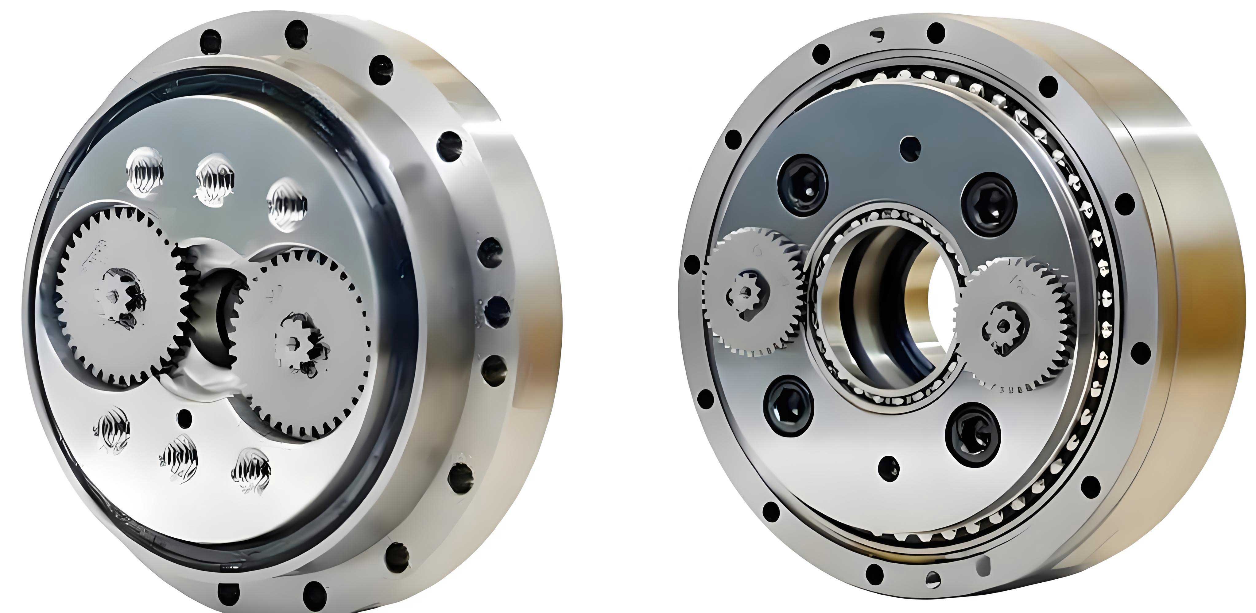
The Rotary Vector (RV) reducer is a high-precision transmission device that serves as a core component in industrial robots. Its transmission accuracy and operational smoothness directly influence the performance of the entire robotic system. During the manufacturing and assembly stages of the RV reducer, geometric errors in critical components are inevitable. These errors, particularly angular misalignments, can significantly degrade transmission precision, reduce operational stability, and adversely affect the service life of the RV reducer. While improving machining quality can mitigate these issues, it often leads to a dramatic increase in cost. Therefore, researching methods to adjust angular errors during the assembly process and to optimally allocate tolerances for key components is of great significance for the cost-effective manufacturing of high-performance RV reducers.
Extensive research exists on tolerance allocation and the transmission accuracy of RV reducers. Prior work has utilized 3D tolerance analysis software, fuzzy analytic hierarchy processes, and adaptive genetic algorithms for tolerance design in complex mechanical systems. For RV reducers specifically, studies have focused on sensitivity analysis of various error sources, dynamic transmission error modeling considering nonlinear factors like wear, and the impact of tooth profile modification. However, a systematic methodology for determining optimal in-process adjustments during the assembly of an RV reducer to compensate for part errors, and subsequently using this adjustment model to inform a cost-optimal tolerance allocation, has not been thoroughly explored. This paper addresses this gap by proposing a comprehensive approach based on state-space modeling and optimal control theory.
The primary performance indicator for an RV reducer is its dynamic transmission error, which quantifies deviations from ideal motion transfer. A smaller transmission error indicates higher precision and smoother operation. The dynamic transmission error, denoted as $$ heta_e(t)$$, is defined as:
$$ heta_e(t) = \frac{ heta_i(t)}{i_z} – heta_o(t)$$
where $$ heta_i(t)$$ is the theoretical input rotation angle, $$i_z$$ is the total reduction ratio, and $$ heta_o(t)$$ is the actual output rotation angle of the RV reducer. The goal of precision assembly is to minimize the final value and variation of $$ heta_e(t)$$ by managing component errors.
The core of the proposed methodology lies in modeling the RV reducer assembly process as a discrete-state system where errors propagate through the assembly sequence. This involves identifying Key Characteristics (KCs), which are critical geometric features whose relative positions determine the final performance of the RV reducer. For a typical RV reducer, the central axes of the crankshafts, cycloid gears, and the pin housing are identified as the primary KCs.
Theoretical Model for Error Propagation
The assembly process is described using a Datum Flow Chain (DFC), which traces the propagation of geometric relationships from a primary datum (e.g., the pin housing axis) to subsequent features. The relative angular deviation of the n-th KC in the chain with respect to the primary datum coordinate system can be represented by a differential rotation vector $$\delta_n$$:
$$\delta_n = [\delta_{x}^{n}, \delta_{y}^{n}, \delta_{z}^{n}]^T$$
This deviation accumulates from the inherent angular error of the newly added part, $$\Delta heta_n = [\Delta heta_{xn}, \Delta heta_{yn}, \Delta heta_{zn}]^T$$, which is defined in its local coordinate system. The transformation between the local part error and the global KC deviation is governed by a matrix $$\mathbf{W}_n$$ that encodes the kinematic relationship between the features in the DFC. Therefore, the propagation can be expressed as:
$$\delta_n = \delta_{n-1} + \mathbf{W}_n \Delta heta_n$$
This incremental error accumulation can be elegantly captured by a state-space model, a powerful framework from control theory. The state vector $$\mathbf{x}(k)$$ at assembly step $$k$$ comprises the differential rotation vectors of all KCs. The state-space equations governing the assembly of the RV reducer are:
$$
\begin{aligned}
\mathbf{x}(k+1) &= \mathbf{A}(k)\mathbf{x}(k) + \mathbf{B}(k)\mathbf{u}(k) + \mathbf{F}(k)\mathbf{w}(k) \\
\mathbf{y}(k) &= \mathbf{C}(k)\mathbf{x}(k) + \mathbf{v}(k)
\end{aligned}
$$
Where:
- $$\mathbf{x}(k)$$: State vector (angular errors of all KCs) at step $$k$$.
- $$\mathbf{A}(k)$$: State transition matrix (typically an identity matrix for rigid assemblies).
- $$\mathbf{B}(k)$$: Control input matrix, mapping adjustment actions to state changes.
- $$\mathbf{u}(k)$$: Control input vector representing deliberate angular adjustments made to the assembly at step $$k$$.
- $$\mathbf{F}(k)$$: Disturbance input matrix, transforming part errors into the state coordinate system.
- $$\mathbf{w}(k)$$: Disturbance vector representing the inherent angular error $$\Delta heta_k$$ of the part added at step $$k$$.
- $$\mathbf{y}(k)$$: Measurement vector (e.g., parallelism between axes measured at step $$k$$).
- $$\mathbf{C}(k)$$: Observation matrix defining which KC relationships are measured.
- $$\mathbf{v}(k)$$: Measurement noise vector.
The matrices $$\mathbf{B}(k)$$ and $$\mathbf{F}(k)$$ are structurally identical when the adjustment and part error are defined in the same coordinate system. The matrix $$\mathbf{F}(k)$$ is a block diagonal matrix composed of the transformation matrices $$\mathbf{W}_{DFC_i}$$ for each independent datum flow chain within the RV reducer assembly.
| Matrix | Role in RV Reducer Assembly | Typical Form / Content |
|---|---|---|
| $$\mathbf{A}(k)$$ | Describes how existing errors propagate to the next state. For rigid assemblies, errors are carried over directly. | Identity Matrix $$\mathbf{I}$$ |
| $$\mathbf{F}(k)$$ | Transforms the native angular error of a newly installed component (e.g., crankshaft, cycloid gear) into the global KC error state. | Block-diag($$\mathbf{W}_{DFC1}, \mathbf{W}_{DFC2}, …$$) |
| $$\mathbf{B}(k)$$ | Defines how a technician’s adjustment action (e.g., shimming, realigning) changes the angular state of the KCs. | Same structure as $$\mathbf{F}(k)$$ for corresponding adjustments. |
| $$\mathbf{C}(k)$$ | Specifies which geometric relationships (e.g., axis of Crankshaft 1 vs. Pin Housing) are verified by measurement during assembly. | Matrix with elements 1, -1, 0. |
Tolerance Allocation Method Based on Optimal Adjustment
The objective during assembly is to achieve the final specified precision for the RV reducer at the lowest possible cost, which includes both part manufacturing cost and assembly adjustment effort. This is formulated as an optimal control problem. We define a quadratic cost function $$J$$ that balances the final assembly accuracy against the effort expended in adjustments:
$$ J = \mathbf{\tilde{y}}^T(N)\mathbf{Q}(N)\mathbf{\tilde{y}}(N) + \sum_{k=0}^{N-1} \left[ \mathbf{\tilde{u}}^T(k)\mathbf{R}(k)\mathbf{\tilde{u}}(k) \right] $$
Where:
- $$\mathbf{\tilde{y}}(N)$$ is the predicted final geometric error of the assembled RV reducer relative to specifications.
- $$\mathbf{Q}(N)$$ is a positive semi-definite weighting matrix that penalizes final geometric inaccuracy. A higher weight in $$\mathbf{Q}(N)$$ places greater importance on that specific geometric perfection of the RV reducer.
- $$\mathbf{\tilde{u}}(k)$$ is the adjustment vector applied at step $$k$$.
- $$\mathbf{R}(k)$$ is a positive definite weighting matrix that penalizes adjustment effort. A high value in $$\mathbf{R}(k)$$ indicates that adjusting a particular KC at that stage is time-consuming or costly.
Minimizing the cost function $$J$$ yields the optimal sequence of adjustments $$\mathbf{u}^*(k)$$ throughout the assembly process of the RV reducer. This optimal control sequence is given by:
$$ \mathbf{u}^*(k) = -\mathbf{K}(k)\mathbf{x}(k) $$
The Kalman gain matrix $$\mathbf{K}(k)$$ is computed recursively backwards from the final step $$N$$:
$$
\begin{aligned}
\mathbf{K}(k) &= [\mathbf{R}(k) + \mathbf{B}^T(k)\mathbf{P}(k+1)\mathbf{B}(k)]^{-1}\mathbf{B}^T(k)\mathbf{P}(k+1)\mathbf{A}(k) \\
\mathbf{P}(k) &= \mathbf{Q}(k) + \mathbf{A}^T(k)\mathbf{P}(k+1)[\mathbf{I} + \mathbf{B}(k)\mathbf{R}^{-1}(k)\mathbf{B}^T(k)\mathbf{P}(k+1)]^{-1}\mathbf{A}(k)
\end{aligned}
$$
with the terminal condition $$\mathbf{P}(N) = \mathbf{Q}(N)$$.
This optimal adjustment strategy provides a direct functional mapping between the final, adjusted error state of the RV reducer and the initial component errors $$\mathbf{w}(k)$$. By running this adjustment policy virtually for many possible component error values (within tolerance bands), we can establish a robust relationship: Final RV Reducer Precision = f(Component Tolerances, Optimal Adjustment).
The tolerance allocation problem can then be framed as an optimization: find the set of component tolerance limits (the maximum allowed values for elements in $$\mathbf{w}(k)$$) that minimize total manufacturing cost while ensuring that, after optimal in-process adjustment, the final RV reducer meets its precision requirement (e.g., a limit on $$ heta_e(t)$$). The manufacturing cost for a component is typically inversely related to the tightness of its tolerance. A common cost-tolerance model is the reciprocal power function:
$$ C_i(t_i) = a_i + \frac{b_i}{t_i^{c_i}} $$
where $$C_i$$ is the cost of manufacturing component $$i$$, $$t_i$$ is its tolerance, and $$a_i, b_i, c_i$$ are fitting parameters.
The complete optimization problem for the RV reducer is:
$$
\begin{aligned}
& \underset{t_1, t_2, …, t_n}{\text{minimize}}
& & \sum_{i=1}^{n} C_i(t_i) \\
& \text{subject to}
& & g_j(\mathbf{t}, \mathbf{u}^*) \leq 0, \quad j = 1, 2, …, m \\
& & & t_i^{L} \leq t_i \leq t_i^{U}
\end{aligned}
$$
where $$g_j(\mathbf{t}, \mathbf{u}^*) \leq 0$$ are the constraints on the final RV reducer performance (e.g., peak-to-peak transmission error, maximum contact stress), which are functions of the tolerances $$\mathbf{t}$$ and the optimal adjustment policy $$\mathbf{u}^*$$. This non-linear constrained optimization problem can be effectively solved using metaheuristic algorithms like the Genetic Algorithm (GA).
| Step | Action | Objective / Outcome |
|---|---|---|
| 1 | Define RV Reducer KCs and Assembly DFC. | Establish the kinematic model for error propagation. |
| 2 | Formulate State-Space Model. | Create matrices $$\mathbf{A}, \mathbf{B}, \mathbf{F}, \mathbf{C}$$ for the assembly sequence. |
| 3 | Define Weights $$\mathbf{Q}(N)$$ and $$\mathbf{R}(k)$$. | Quantify the cost of final inaccuracy vs. adjustment effort. |
| 4 | Compute Optimal Adjustment Gain $$\mathbf{K}(k)$$. | Derive the optimal in-process adjustment policy for the RV reducer. |
| 5 | Establish Cost-Tolerance Models $$C_i(t_i)$$. | Define the relationship between machining cost and tolerance for each part. |
| 6 | Formulate & Solve Optimization Problem via GA. | Find the set of tolerances that minimizes total cost while guaranteeing final RV reducer precision after optimal adjustment. |
Case Study: BX40E-Type RV Reducer
To demonstrate the methodology, a BX40E-type RV reducer is analyzed. The model is simplified to a 2D plane for clarity, considering angular errors around one axis only. Four KCs are defined: the axes of the two crankshafts (KC1, KC3) and the axes of the two cycloid gears (KC2, KC4), relative to the pin housing datum (KC0). The state vector is $$\mathbf{x} = [\delta_1, \delta_2, \delta_3, \delta_4]^T$$. The state transition equation, relating KC deviations to part errors $$\Delta heta_1$$ to $$\Delta heta_4$$, is:
$$
\begin{bmatrix}
\delta_1 \\ \delta_2 \\ \delta_3 \\ \delta_4
\end{bmatrix}
=
\begin{bmatrix}
1 & 0 & 0 & 0 \\
1 & 1 & 0 & 0 \\
0 & 0 & 1 & 0 \\
0 & 0 & 1 & 1
\end{bmatrix}
\begin{bmatrix}
\Delta heta_1 \\ \Delta heta_2 \\ \Delta heta_3 \\ \Delta heta_4
\end{bmatrix}
$$
Thus, the matrices $$\mathbf{A}$$ and $$\mathbf{F}$$ in the state-space model are derived accordingly. The assembly sequence is defined as four steps: install KC1, KC2, KC3, then KC4.
Adjustment matrices $$\mathbf{T}(k)$$ (which parts can be adjusted at step $$k$$) and effort weight matrices $$\mathbf{R}(k)$$ are defined. For example, at step 1, only KC1 can be adjusted with a moderate effort weight of 5, while other uninstalled KCs are given a prohibitively high weight of 1000. The final observation matrix $$\mathbf{C}(4)$$ checks the parallelism of the two crankshaft axes and the two cycloid gear axes relative to the housing datum. The final accuracy weight $$\mathbf{Q}(4)$$ is set to a diagonal matrix with a value $$Q$$, where a higher $$Q$$ imposes a stricter penalty on final geometric error.
| Component Error | $$\Delta heta_1$$ | $$\Delta heta_2$$ | $$\Delta heta_3$$ | $$\Delta heta_4$$ |
|---|---|---|---|---|
| Value (mrad) | -1.6 | 5.3 | 5.8 | 3.2 |
Using the recursive equations, the optimal adjustment gain matrices $$\mathbf{K}(k)$$ are calculated. For a given $$Q$$ value (e.g., $$Q=10$$), the optimal adjustments $$\mathbf{u}^*(k)$$ at each step are computed based on the simulated state $$\mathbf{x}(k)$$. This process effectively reduces the final geometric error state of the RV reducer. The impact of the final accuracy weight $$Q$$ is significant. As $$Q$$ increases, the optimal adjustment policy prioritizes final precision over adjustment effort, leading to a final assembly state closer to the ideal (zero error).
The effectiveness is evaluated by simulating the dynamic transmission error $$ heta_e(t)$$ and the dynamic meshing forces within the RV reducer for different $$Q$$ values. The results show that with optimal adjustment enabled ($$Q > 0$$), both the fluctuation amplitude of the transmission error and the peak meshing forces are substantially reduced compared to the unadjusted case ($$Q=0$$), indicating improved precision and smoothness for the RV reducer. However, the rate of improvement diminishes as $$Q$$ becomes very large, indicating a point of diminishing returns.
| Accuracy Weight (Q) | Transmission Error Peak-to-Peak Amplitude (arc-sec) | Reduction vs. Q=0 | Maximum Dynamic Meshing Force (N) | Reduction vs. Q=0 |
|---|---|---|---|---|
| 0 (No Adjustment) | 52.3 | 0% | 1245 | 0% |
| 5 | 18.7 | 64.2% | 892 | 28.4% |
| 10 | 15.1 | 71.1% | 865 | 30.5% |
| $$\infty$$ (Ideal Target) | 12.5 | 76.1% | 842 | 32.4% |
This state-space and optimal adjustment model establishes a direct functional relationship between the final, adjusted KC errors ($$\delta_i$$) and the original component machining errors ($$v_{jx}$$, etc.). For the BX40E model, this relationship can be simplified to a linear mapping:
$$
\begin{aligned}
P_1 &= 0.3069 v_{1x}, \quad P_2 = 0.3069 v_{1y}, … \\
P_4 &= 0.0491 v_{1x} + 0.1514 v_{2x}, \quad …
\end{aligned}
$$
where $$P_i$$ represent the final KC error states that influence RV reducer performance. Using a Genetic Algorithm with the reciprocal cost function $$C_i = a_i + b_i / t_i$$, the optimal tolerance allocation that minimizes total manufacturing cost while ensuring the final adjusted KC errors (and thus transmission error) meet specifications can be found.
| Component | Optimal Angular Tolerance (mrad) | ||
|---|---|---|---|
| X-axis ($$t_{ix}$$) | Y-axis ($$t_{iy}$$) | Z-axis ($$t_{iz}$$) | |
| Crankshaft 1 | 1.71 | 1.66 | 1.69 |
| Cycloid Gear 1 | 2.63 | 2.62 | 2.62 |
| Crankshaft 2 | 1.54 | 1.52 | 1.52 |
| Cycloid Gear 2 | 1.26 | 1.26 | 1.26 |
Discussion and Implications
The proposed methodology integrates assembly process planning, in-process metrology and adjustment, and design-stage tolerance allocation into a coherent framework for the RV reducer. The state-space model provides a precise, quantitative description of how part errors propagate, which is superior to traditional worst-case or statistical stack-up analyses that often ignore the possibility of corrective actions during assembly.
The choice of the final accuracy weight $$Q$$ is critical. It acts as a tuning parameter that balances the conflicting objectives of product quality and assembly cost. A very high $$Q$$ will force the optimal adjustment to chase perfection, potentially requiring very precise and time-consuming adjustments, which increases assembly cost. A lower $$Q$$ saves on adjustment effort but accepts a larger final geometric error in the RV reducer. The relationship between $$Q$$ and final performance is nonlinear, showing diminishing returns. Therefore, selecting $$Q$$ should be based on a clear understanding of the required performance specifications for the RV reducer and the associated cost structures.
The tolerance allocation results (Table 5) are not uniform. The algorithm assigns tighter tolerances to components whose errors have a higher sensitivity in the final adjusted state (e.g., Crankshaft 2 and Cycloid Gear 2 in this case study) and looser tolerances to less sensitive components. This non-uniform allocation is the key to cost savings, as it avoids overspending on tightening tolerances unnecessarily while ensuring the overall RV reducer performance target is met through the optimal adjustment strategy.
| Aspect | Advantage |
|---|---|
| Accuracy Prediction | Provides a dynamic, step-by-step prediction of geometric error state, enabling proactive adjustment. |
| Process Guidance | Generates an optimal adjustment sequence, telling the assembler *what* to adjust and *by how much* at each step. |
| Cost-Optimal Tolerancing | Links assembly adjustment capability directly to design tolerances, finding the least-cost combination that guarantees final RV reducer quality. |
| Flexibility | The model can be adapted to different RV reducer architectures and assembly sequences by redefining the DFC and matrices. |
In practical implementation, the success of this method relies on accurate measurement of the KC relationships at specified assembly steps. The measurement noise $$v(k)$$ in the model accounts for this uncertainty. Furthermore, the cost-tolerance models $$C_i(t_i)$$ must be calibrated with real manufacturing data from the supply chain to ensure the economic validity of the optimization results.
Conclusion
This paper presents a systematic methodology for enhancing the precision of Rotary Vector (RV) reducers through optimal in-process angular error adjustment and cost-driven tolerance allocation. By modeling the RV reducer assembly as a state-space system, the propagation of component errors is rigorously described. The application of optimal control theory yields a sequence of adjustments that optimally compensates for these errors, balancing the final geometric quality of the RV reducer against the effort required for adjustment.
The critical finding is that the final performance of the RV reducer is not solely determined by part tolerances, but by the combination of tolerances and the applied adjustment strategy. This allows for the intentional allocation of looser, less expensive tolerances on certain components, provided that a planned, optimal adjustment compensates for the resulting errors during assembly. The use of a Genetic Algorithm efficiently solves the resulting non-linear cost optimization problem, providing a pragmatic set of component tolerances.
The case study on a BX40E-type reducer validates the approach, showing significant reduction in simulated transmission error and dynamic forces when the optimal adjustment policy is applied. The analysis of the accuracy weight parameter $$Q$$ provides valuable guidance for manufacturers, indicating that while higher precision is achievable, the marginal cost increases, and an optimal operating point must be chosen based on specific product requirements. This integrated approach provides a powerful and practical framework for the design and manufacture of high-precision, cost-competitive RV reducers.