
As a researcher focused on precision machinery, I have extensively studied the vibration behavior of RV reducers, which are critical components in industrial robots. The performance of these RV reducers directly impacts the end-effector accuracy, making it essential to understand their vibration characteristics. In this article, I present a comprehensive analysis based on experimental data, employing autocorrelation techniques to delve into the correlation of vibration signals. My goal is to provide insights that can aid in fault diagnosis and performance enhancement for RV reducers. Throughout this work, I emphasize the importance of the RV reducer in robotic systems and explore how its vibrational properties evolve under varying operational conditions.
The vibration analysis of RV reducers is a complex task due to their multi-stage transmission design. Typically, an RV reducer consists of a first-stage involute planetary gear system and a second-stage cycloidal pin-wheel system. This structure introduces multiple meshing frequencies and rotational components that contribute to the overall vibration signature. To capture these dynamics, I designed a series of tests on an RV-40E reducer, which is widely used in industrial applications. The experiments involved constant-speed, acceleration, and deceleration scenarios, with vibration signals collected across different input speeds. By applying frequency domain analysis and autocorrelation analysis, I aimed to identify characteristic frequencies and assess their influence on the RV reducer’s operation. The findings from this study underscore the value of autocorrelation methods in revealing hidden periodicities and trends in vibration data for RV reducers.
In this investigation, I utilized a precision reducer comprehensive test platform to evaluate the RV reducer. The setup included a drive motor, torque sensor, bearing seats, angular sensors, and the RV reducer under test. Vibration signals were acquired using a vibration signal analyzer and a data acquisition card, with uniaxial accelerometers mounted at strategic points on the RV reducer’s housing. Specifically, I placed sensors in the X, Y, and Z directions to capture multi-axis vibrations. This arrangement allowed me to gather data under various conditions: input speeds of 500 r/min, 1000 r/min, 1500 r/min, 1815 r/min, as well as during acceleration from 0 to 1815 r/min and deceleration from 1815 to 0 r/min. All data processing was performed using MATLAB, where I implemented algorithms for fast Fourier transform (FFT) and autocorrelation computation. The autocorrelation function, which measures the similarity between a signal and its time-lagged version, is defined as:
$$R_{xx}(\tau) = \lim_{T \to \infty} \frac{1}{T} \int_{-T/2}^{T/2} x(t) x(t + \tau) dt$$
For discrete signals, this can be approximated as:
$$R_{xx}[k] = \sum_{n=0}^{N-1} x[n] x[n + k]$$
where \( x(t) \) is the vibration signal, \( \tau \) is the time lag, \( T \) is the observation period, and \( k \) represents the lag index. This mathematical tool helps in filtering out noise and extracting periodic components, making it ideal for analyzing the RV reducer’s vibration characteristics.
The RV-40E reducer has specific geometric parameters that determine its characteristic frequencies. The first-stage involves a sun gear with tooth number \( z_1 = 12 \) and planetary gears with \( z_2 = 36 \). The second-stage includes a cycloid gear with tooth number \( z_4 = 39 \) and a pin gear with \( z_5 = 40 \). Based on these, the theoretical characteristic frequencies can be calculated using the following formulas, where \( n_0 \) is the output speed in r/min and \( n_1 \) is the input speed in r/min:
- Sun gear rotational frequency: \( f_1 = \frac{n_1}{60} \)
- First-stage meshing frequency: \( f_{1c} = z_1 \cdot f_1 = \frac{n_1 \cdot z_1}{60} \)
- Planetary gear meshing frequency: \( f_{\text{gear}} = \frac{n_0 \cdot z_2 \cdot (z_5 – 1)}{60} \)
- Second-stage meshing frequency: \( f_{2c} = \frac{z_1 \cdot z_4 \cdot f_1}{z_2} = \frac{n_1 \cdot z_1 \cdot z_4}{60 \cdot z_2} \)
- Cycloid gear rotational frequency: \( f_0 = \frac{n_0}{60} \)
- Pin gear characteristic frequency: \( f_3 = \frac{2n_0 \cdot (z_5 – 1)}{60 \cdot z_5} \)
- Planetary gear rotational frequency: \( f_2 = \frac{n_0 \cdot (z_5 – 1)}{60} \)
- Pin meshing frequency: \( f_{\text{pin}} = \frac{2n_0 \cdot (z_5 – 1)}{60} \)
To provide a clear overview, I computed these frequencies for the tested input speeds, as summarized in the table below. The values highlight how the characteristic frequencies scale with speed, which is crucial for interpreting the vibration spectra of the RV reducer.
| Input Speed (r/min) | \( f_1 \) (Hz) | \( f_{1c} \) (Hz) | \( f_{\text{gear}} \) (Hz) | \( f_{2c} \) (Hz) | \( f_0 \) (Hz) | \( f_3 \) (Hz) | \( f_2 \) (Hz) | \( f_{\text{pin}} \) (Hz) |
|---|---|---|---|---|---|---|---|---|
| 500 | 8.33 | 100.00 | 96.69 | 108.33 | 0.069 | 0.130 | 2.69 | 5.37 |
| 1000 | 16.67 | 200.00 | 193.39 | 226.67 | 0.138 | 0.270 | 5.37 | 10.74 |
| 1500 | 25.00 | 300.00 | 290.08 | 325.00 | 0.207 | 0.403 | 8.06 | 16.12 |
| 1815 | 30.25 | 363.00 | 351.00 | 393.25 | 0.250 | 0.4875 | 9.75 | 19.50 |
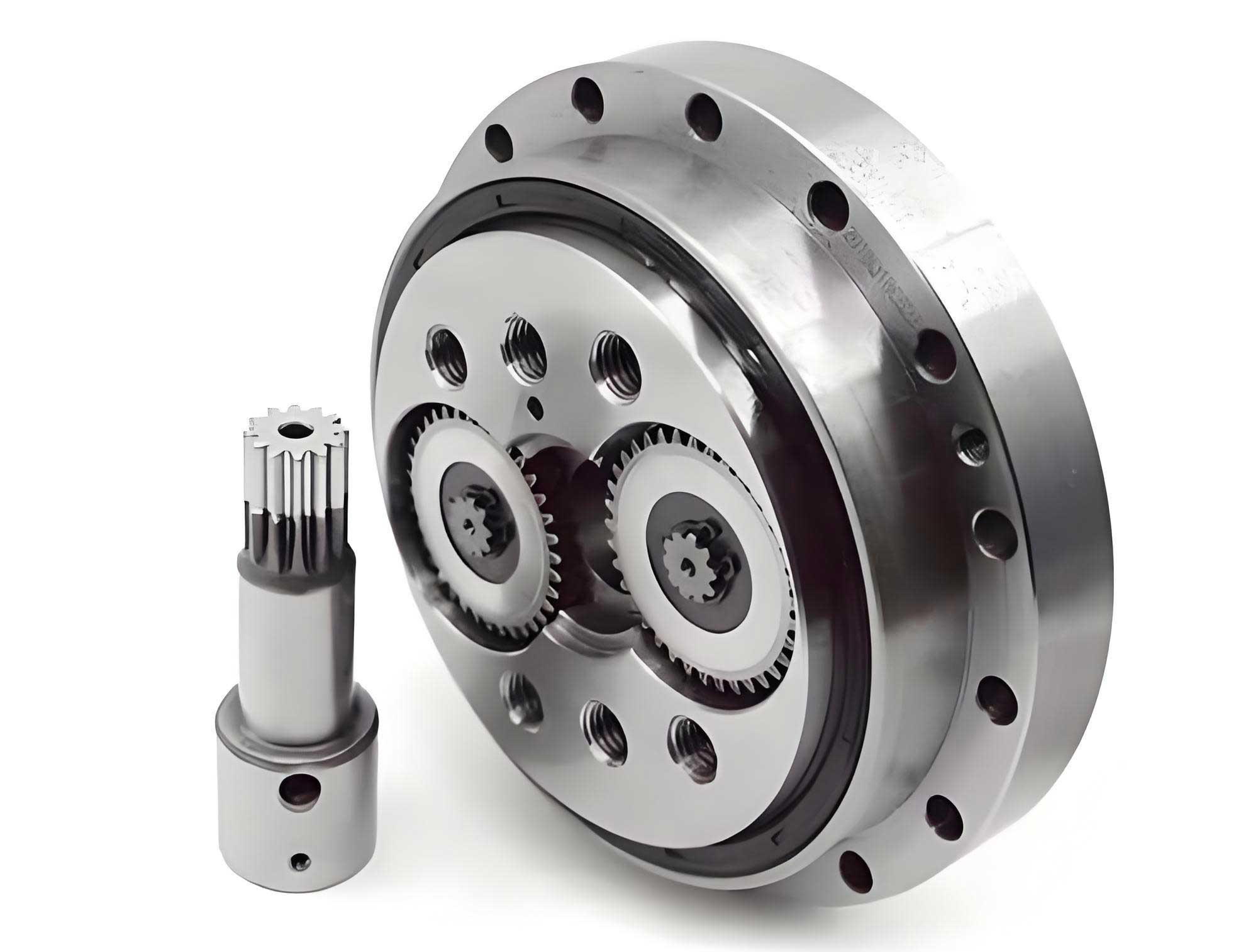
To visualize the RV reducer’s structure, which aids in understanding its vibration sources, I include the following image link. This depiction shows the internal gearing arrangement of a typical RV reducer, highlighting the planetary and cycloidal stages that contribute to its complex dynamics.
In the constant-speed tests, I analyzed the vibration signals at 500 r/min, 1000 r/min, 1500 r/min, and 1815 r/min. For each case, I performed spectral analysis to identify frequency components and autocorrelation analysis to assess periodicity and signal consistency. At 500 r/min, the spectrum revealed a series of high-amplitude peaks at 25 Hz, 75 Hz, 125 Hz, 175 Hz, 225 Hz, and 275 Hz. These frequencies, spaced at 50 Hz intervals, were attributed to electrical interference rather than mechanical sources of the RV reducer. Among the characteristic frequencies, I detected the sun gear rotational frequency \( f_1 \) at 8.6 Hz and the second-stage meshing frequency \( f_{2c} \) at 110 Hz. Comparing these with theoretical values from Table 1, the errors were minimal, indicating accurate measurement. The autocorrelation plot showed prominent peaks occurring approximately every 0.8 seconds, corresponding to a frequency of 1.25 Hz. This periodicity suggested a stable vibration pattern at this speed for the RV reducer, with autocorrelation coefficients remaining consistent over time.
Increasing the speed to 1000 r/min, the spectral analysis displayed similar electrical noise peaks, but the characteristic frequencies became more pronounced. Specifically, \( f_{2c} \) appeared at 226.8 Hz, \( f_{\text{gear}} \) at 194 Hz, and \( f_{1c} \) at 200.2 Hz. The errors relative to theoretical values were below 0.5%, as detailed in the following error analysis table for the RV reducer. Notably, the amplitudes of these meshing frequencies increased significantly compared to the 500 r/min case, underscoring their sensitivity to speed changes in the RV reducer.
| Characteristic Frequency | Theoretical Value (Hz) | Experimental Value (Hz) | Error (%) |
|---|---|---|---|
| \( f_{2c} \) | 226.67 | 226.80 | 0.06 |
| \( f_{\text{gear}} \) | 193.39 | 194.00 | 0.32 |
| \( f_{1c} \) | 200.00 | 200.80 | 0.40 |
The autocorrelation analysis at 1000 r/min also revealed peaks at 0.8-second intervals, but with greater stability and higher correlation values than at 500 r/min. This enhancement in autocorrelation strength indicates that the RV reducer’s vibration signals become more periodic and predictable as speed rises. The consistency of the 0.8-second period across speeds suggests a underlying mechanical rhythm, possibly related to the rotational dynamics of the RV reducer’s components.
At 1500 r/min, the spectral peaks at 125 Hz and 175 Hz grew markedly in amplitude, likely due to resonance effects. The characteristic frequencies \( f_1 \), \( f_{2c} \), and \( f_{1c} \) aligned perfectly with theoretical values, as shown in the error table below for the RV reducer. The amplitude of \( f_{2c} \) saw a substantial rise, highlighting its dominance in the vibration spectrum at higher speeds for the RV reducer.
| Characteristic Frequency | Theoretical Value (Hz) | Experimental Value (Hz) | Error (%) |
|---|---|---|---|
| \( f_1 \) | 25.00 | 25.00 | 0.00 |
| \( f_{2c} \) | 325.00 | 325.00 | 0.00 |
| \( f_{1c} \) | 300.00 | 300.20 | 0.07 |
The autocorrelation plot maintained the 0.8-second peak periodicity, reinforcing the notion of a speed-invariant rhythmic pattern in the RV reducer’s vibrations. This persistence across speeds suggests that this periodicity may stem from structural modes or assembly characteristics of the RV reducer, rather than direct speed-dependent phenomena.
At the maximum tested speed of 1815 r/min, the spectral analysis showed a prominent peak at 150 Hz, along with identifiable characteristic frequencies. The values for \( f_{2c} \), \( f_2 \), \( f_1 \), and \( f_{\text{gear}} \) matched theoretical predictions with errors under 1.2%, as summarized in the table below for the RV reducer. However, their amplitudes were relatively low, indicating that at this speed, other factors such as electrical noise or system resonances might overshadow the mechanical vibration signatures of the RV reducer.
| Characteristic Frequency | Theoretical Value (Hz) | Experimental Value (Hz) | Error (%) |
|---|---|---|---|
| \( f_{2c} \) | 393.25 | 393.90 | 0.17 |
| \( f_2 \) | 9.75 | 9.80 | 0.51 |
| \( f_1 \) | 30.25 | 30.60 | 1.16 |
| \( f_{\text{gear}} \) | 351.00 | 352.00 | 0.28 |
The autocorrelation analysis again displayed the 0.8-second periodicity, confirming that this feature is robust across the operational range of the RV reducer. Comparing all constant-speed cases, I observed that as speed increases, the autocorrelation of the RV reducer’s vibration signals strengthens, implying greater signal regularity and potentially lower noise contamination.
In the dynamic tests, where the RV reducer was accelerated from 0 to 1815 r/min and decelerated from 1815 to 0 r/min, the vibration behavior differed. During acceleration, the spectrum showed characteristic frequencies such as \( f_{2c} \) at 325 Hz, \( f_{\text{gear}} \) at 290.08 Hz, \( f_2 \) at 5.37 Hz, and \( f_1 \) at 25 Hz, but their amplitudes did not exhibit clear trends due to the transient nature. The autocorrelation plot revealed peaks at 0.8-second intervals, similar to constant speeds, but with additional minor peaks every 0.4 seconds (corresponding to 2.5 Hz). This suggests that during acceleration, the RV reducer experiences extra vibrational modes, possibly from inertial effects or changing meshing conditions. In contrast, during deceleration, the autocorrelation coefficients fluctuated around zero without distinct periodicity, indicating a loss of signal consistency. This absence of periodicity in deceleration aligns with the notion that the RV reducer’s vibration characteristics are less stable during speed reductions, which could be critical for fault detection in real-world applications.
To further analyze the impact of speed on the RV reducer, I plotted the amplitude variations of key characteristic frequencies across different speeds. The trends show that \( f_1 \), \( f_{1c} \), and \( f_{2c} \) peak in amplitude at 1500 r/min, then slightly decrease at 1815 r/min. This non-linear behavior may relate to resonance frequencies or system damping within the RV reducer. Additionally, the electrical noise frequencies (25 Hz, 75 Hz, 125 Hz, etc.) exhibited their own patterns, with 75 Hz consistently having the highest amplitude. These observations underscore the complexity of vibration sources in the RV reducer, where mechanical and electrical components interact.
From a theoretical perspective, the autocorrelation function’s behavior can be modeled using the equation for a periodic signal with noise. If the vibration signal \( x(t) \) is composed of a periodic component \( p(t) \) and random noise \( n(t) \), such that \( x(t) = p(t) + n(t) \), then the autocorrelation is:
$$R_{xx}(\tau) = R_{pp}(\tau) + R_{nn}(\tau) + 2R_{pn}(\tau)$$
Assuming the noise is uncorrelated with the periodic signal, \( R_{pn}(\tau) = 0 \), and for white noise, \( R_{nn}(\tau) \) approaches zero for \( \tau > 0 \). Thus, \( R_{xx}(\tau) \approx R_{pp}(\tau) \) for non-zero lags, revealing the periodicities in the RV reducer’s vibration. This mathematical foundation explains why autocorrelation analysis effectively extracts repetitive features from the noisy signals of the RV reducer.
In terms of practical implications, the findings from this study on the RV reducer have several key takeaways. First, the autocorrelation strength increases with speed, suggesting that at higher operational speeds, the RV reducer’s vibrations become more predictable, which could be advantageous for monitoring systems. Second, the consistent 0.8-second periodicity across speeds points to a structural or assembly-related frequency that might be used as a baseline for health assessment of the RV reducer. Third, the meshing frequencies \( f_{1c} \) and \( f_{2c} \) show significant amplitude changes with speed, indicating they are major contributors to the vibrational energy in the RV reducer. This makes them prime candidates for fault diagnosis, as deviations from expected patterns could signal wear or misalignment in the RV reducer.
To encapsulate the overall trends, I compiled a summary table of amplitude changes for the primary characteristic frequencies across the tested speeds for the RV reducer. This table highlights how each frequency evolves, providing a quick reference for engineers working with RV reducers.
| Characteristic Frequency | 500 r/min Amplitude | 1000 r/min Amplitude | 1500 r/min Amplitude | 1815 r/min Amplitude | Trend |
|---|---|---|---|---|---|
| \( f_1 \) (Sun gear rotational) | Low | Medium | High | Medium | Increases then decreases |
| \( f_{1c} \) (First-stage meshing) | Low | Medium | High | Low | Peaks at 1500 r/min |
| \( f_{2c} \) (Second-stage meshing) | Low | High | Very High | Medium | Increases significantly with speed |
| \( f_{\text{gear}} \) (Planetary meshing) | Low | Medium | High | Medium | Generally increases |
| Electrical Noise (75 Hz) | High | Very High | Very High | High | Consistently dominant |
In conclusion, this comprehensive analysis of the RV reducer demonstrates the efficacy of autocorrelation methods in vibration characterization. The RV reducer’s vibrational behavior is intricately linked to its design parameters and operational speeds, with meshing frequencies playing a pivotal role. The autocorrelation analysis not only revealed periodicities but also showed that signal consistency improves at higher speeds for the RV reducer. These insights can inform condition monitoring strategies and predictive maintenance for RV reducers in industrial robots. Future work could explore the effects of load variations or different RV reducer models to broaden the understanding. Ultimately, mastering the vibration characteristics of RV reducers through techniques like autocorrelation will enhance their reliability and performance in demanding applications.