
The RV reducer, a two-stage reduction mechanism combining cycloidal-pin gear and involute planetary gear drives, is a cornerstone of modern precision motion systems. Its key advantages include a high transmission ratio, substantial load-bearing capacity, excellent rigidity, compact size, minimal backlash, high motion accuracy, and superior transmission efficiency. As a result, the RV reducer has become the preferred transmission solution for critical applications such as industrial robot joints. With growing domestic market demand and the strategic importance of high-precision manufacturing, extensive research and prototype development are underway. However, achieving the RV reducer’s theoretical performance in mass production presents significant challenges. Its structure is statically indeterminate, involving numerous components. While the cycloidal drive theoretically engages with half the pin teeth simultaneously for near-zero backlash and high load sharing, practical manufacturing introduces errors. Factors like machining tolerances, geometric imperfections, and assembly variations can disrupt this ideal multi-tooth conjugate contact. Traditional two-dimensional tolerance stack-up analysis often fails to capture the complex three-dimensional spatial relationships and constraints between components. Furthermore, prevalent reliance on manual fitting and adjustment in production severely impacts efficiency and consistency. This article details a methodology for static assembly tolerance analysis and optimization of an RV reducer using three-dimensional Computer-Aided Tolerancing (3D CAT) software, 3DCS, integrated within the CATIA V5 environment. This approach simulates real-world assembly conditions, enabling optimization of component tolerances while guaranteeing final product performance and assembly yield.
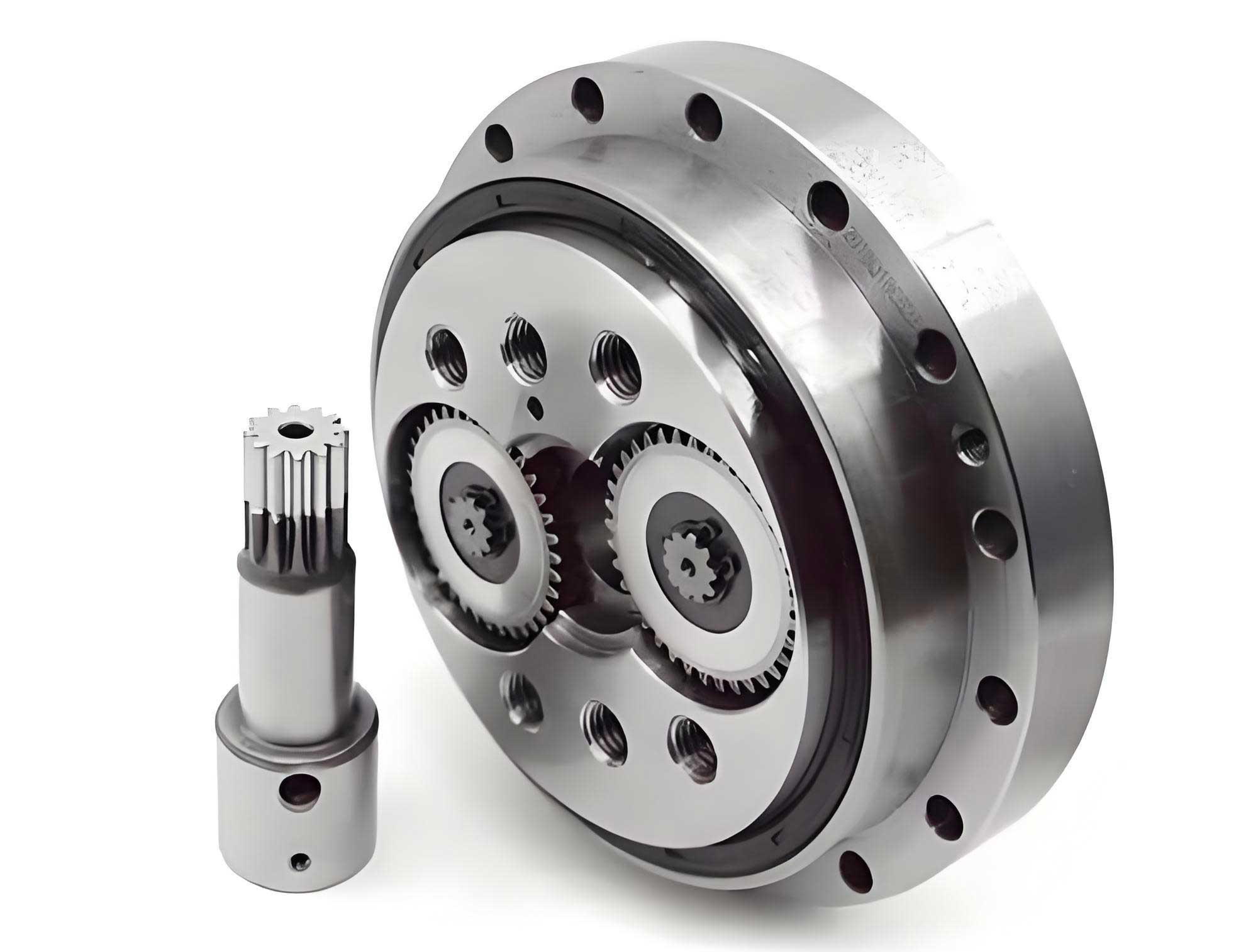
The typical RV reducer configuration, such as the RV-40E-81 model, integrates a first-stage involute planetary gear train and a second-stage cycloidal-pin gear train. It commonly features two or three planetary gears and a pair of cycloidal wheels mounted 180° apart on multiple crankshafts. This design, along with the use of needle roller bearings on the crankshafts, enables effective power splitting, enhances bearing life, and increases overall torsional stiffness. The output is connected to an output flange (or support plate) which houses the crankshaft bearings. The entire assembly is enclosed within a rigid pin housing, supported by large main bearings. To analyze the dimensional relationships critical for assembly and performance, an assembly dimension chain must be established. For the static assembly analysis focusing on the second-stage cycloidal drive, the key dimensions and their interactions are illustrated in the figure below.
The fundamental equations governing the geometric relationships within the RV reducer’s cycloidal stage, ignoring bearing internal clearances for the initial model, are as follows:
$$ a = L_1 + a_1 – L_2 $$
$$ \Delta_1 = r_a – r_f – r_p $$
$$ \Delta_2 = r_p + r_{pp} – r_a $$
$$ \Delta_3 = r_1 + r_2 + a_1 – L_2 $$
In these equations, $a$ represents the theoretical eccentricity, $L_1$ is the distance from the geometric center of the output/support plate to the center of its crankshaft bearing bore, $a_1$ is the crankshaft’s eccentric offset, and $L_2$ is the distance from the geometric center of the cycloidal wheel to the center of its needle roller bore. For the pin gear set, $r_p$ is the radius of the pin (needle), $r_{pp}$ is the radius of the pin distribution circle (the center circle on which all pins are mounted), $r_a$ is the tip circle radius of the cycloidal wheel tooth, and $r_f$ is its root circle radius. $\Delta_1$ and $\Delta_2$ represent radial clearances. The final equation involves the first stage, where $r_1$ and $r_2$ are the reference radii of the sun gear (on the input shaft) and the planetary gear, respectively, but this stage’s constraints are neglected in the primary static assembly model for the cycloidal drive.
A critical component for the RV reducer’s performance is the cycloidal wheel. Its tooth profile is defined by a modified trochoidal equation. The parametric equations used for 3D modeling, accounting for profile modification (shift and equidistance), are given by:
$$ x = (r_{pp} + \Delta r_{pp}) \sin \psi – a \sin(z_p \psi) + (r_p + \Delta r_p) \times $$
$$ \left[ K \sin \psi – \frac{\sin(z_c \psi)}{z_p} \right] / \left[ 1 + K^2 – 2K \cos(z_c \psi) \right]^{1/2} $$
$$ y = (r_{pp} + \Delta r_{pp}) \cos \psi – a \cos(z_p \psi) + (r_p + \Delta r_p) \times $$
$$ \left[ K \cos \psi – \frac{\cos(z_c \psi)}{z_p} \right] / \left[ 1 + K^2 – 2K \cos(z_c \psi) \right]^{1/2} $$
where, $$ K = 1 – (a z_c) / (r_{pp} + \Delta r_{pp}) \cdot \cos(z_c \psi) $$
In these equations, $\psi$ is the generating angle (in radians, from $0$ to $2\pi$), $z_c$ is the number of cycloidal wheel teeth, $z_p$ is the number of pin teeth, $\Delta r_{pp}$ is the profile shift modification amount, and $\Delta r_p$ is the equidistant modification amount. The modifications $\Delta r_{pp}$ and $\Delta r_p$ are crucial for ensuring proper lubrication and compensating for errors, but they must be tightly controlled to preserve the multi-tooth contact characteristic essential for the RV reducer’s high stiffness and load capacity.
The core of this analysis lies in building a complete 3DCS tolerance simulation model. This model comprises four main elements: the 3D geometric models of all parts, the application of dimensional and geometric tolerances to these parts, the definition of the assembly sequence and mating constraints, and finally, the specification of measurement features. Using CATIA V5, detailed solid models were created for all components: the pin housing, pins, crankshaft, cycloidal wheels, output flange, support plate, and bearings. The cycloidal wheel was modeled parametrically using the equations above, with each tooth profile as an independent feature to allow for the application of individual profile errors. This detailed modeling is fundamental for an accurate RV reducer simulation.
The next step is tolerance assignment. Based on preliminary design specifications and the assembly dimension chain analysis, critical tolerances were defined for key features. These include dimensions like the pin circle radius $r_{pp}$, crankshaft eccentricity $a_1$, and distances $L_1$ and $L_2$, as well as geometric tolerances such as the coaxiality of the main bearing bores in the pin housing, the position of pin holes, and runout/accumulative pitch error of the cycloidal wheel teeth. The initial tolerance values (pre-optimization) for major components are summarized in Table 1. In 3DCS, these tolerances are applied directly to the 3D geometry, defining how each feature can vary within its specified range.
| Component | Feature Name | Basic Size (mm) | Deviation (mm) | Tolerance (mm) |
|---|---|---|---|---|
| Pin Housing | Main Bearing Bore Coaxiality | – | 0 | 0.010 |
| Pin Housing | Pin Hole Circumferential Position | – | 0 | 0.006 |
| Pin Housing | Pin Distribution Circle Radius, $r_{pp}$ | 66 | 0 | 0.002 |
| Pin | Pin Radius, $r_p$ | 3 | -0.003 | 0.002 |
| Output/Support Plate | Crankshaft Bore Center Distance, $L_1$ | 72 | 0 | 0.012 |
| Crankshaft | Crank Eccentricity, $a_1$ | 1.25 | 0 | 0.006 |
| Cycloidal Wheel | Needle Bore Center Distance, $L_2$ | 72 | 0 | 0.012 |
| Cycloidal Wheel | Shift Modification, $\Delta r_{pp}$ | -0.014 | 0 | 0.004 |
| Cycloidal Wheel | Equidistant Modification, $\Delta r_p$ | -0.012 | 0 | 0.002 |
| Cycloidal Wheel | Tooth Ring Radial Runout | – | 0.00375 | 0.0075 |
| Cycloidal Wheel | Accumulative Pitch Error | – | 0.005 | 0.009 |
| – | Theoretical Eccentricity, $a$ | 1.25 | 0 | 0.010 |
Defining the assembly sequence and mating conditions in 3DCS is crucial for simulating real-world assembly. The sequence must reflect the hierarchical relationship of parts and sub-assemblies. For the RV reducer, a typical sequence might start with fixing the pin housing, then installing the main bearings, followed by the output flange assembly (with crankshafts and cycloidal wheels pre-assembled), and finally the support plate. Mates such as concentricity (for bearings in bores), surface contact (for flange against bearing face), and distance offsets (for crankshaft eccentricity) are defined to replicate the physical assembly constraints accurately.
Finally, critical measurement parameters are established to evaluate the assembly outcome. For the RV reducer, two key measurements are defined: 1) Eccentricity Error: The distance between the geometric center of the assembled cycloidal wheel set (considered as a floating component) and the geometric center of the pin housing. This deviation from the theoretical eccentricity $a$ affects the fundamental kinematics of the cycloidal drive. 2) Tooth Flank Clearance: The minimum distance between the flank of a cycloidal tooth and the surface of its corresponding pin at the theoretical point of contact. This clearance is measured for multiple pin/cycloidal tooth pairs around the circumference to ensure there is no interference and that a small, positive clearance exists for lubrication. A clearance greater than or equal to 0.001 mm is typically targeted to ensure assemblability while minimizing backlash. The backlash of the entire RV reducer, a critical performance metric, can be derived from the pattern of these individual flank clearances.
With the complete 3DCS model, Monte Carlo simulation is performed. This method randomly generates thousands of component instances based on their defined tolerance distributions and assembles them virtually according to the specified sequence. The measurement parameters (eccentricity and flank clearances) are calculated for each virtual assembly. The statistical results, analyzed using the Six Sigma (6σ) principle, reveal the assembly yield. The initial simulation with the tolerances from Table 1 showed significant issues. Approximately 3.78% of assemblies had eccentricity errors outside the acceptable range. More critically, a high percentage of assemblies showed flank clearance violations (less than 0.001 mm or interference) at specific teeth: 14.8% at tooth #3, 26.7% at tooth #6, and 14.8% at tooth #9. This indicated an unacceptably low assembly yield for a high-precision component like the RV reducer.
To address this, an iterative tolerance optimization process was conducted within 3DCS. The software’s sensitivity analysis feature identifies which tolerances contribute most significantly to the variation in each measurement. Based on this feedback, tolerances were tightened on the most sensitive features and, where possible, loosened on less sensitive ones to maintain a cost-effective manufacturing profile. The optimization goal was to ensure 100% of simulated assemblies met the eccentricity requirement and all flank clearances were ≥0.001 mm, resulting in a final calculated backlash range of 0.25 to 1 arc-minute, which meets typical performance specifications for an RV reducer. The optimized tolerance values are presented in Table 2.
| Component | Feature Name | Basic Size (mm) | Deviation (mm) | Tolerance (mm) |
|---|---|---|---|---|
| Pin Housing | Main Bearing Bore Coaxiality | – | 0 | 0.005 |
| Pin Housing | Pin Hole Circumferential Position | – | 0 | 0.005 |
| Pin Housing | Pin Distribution Circle Radius, $r_{pp}$ | 66 | -0.002 | 0.002 |
| Pin | Pin Radius, $r_p$ | 3 | -0.006 | 0.001 |
| Output/Support Plate | Crankshaft Bore Center Distance, $L_1$ | 72 | 0 | 0.010 |
| Crankshaft | Crank Eccentricity, $a_1$ | 1.25 | 0 | 0.004 |
| Cycloidal Wheel | Needle Bore Center Distance, $L_2$ | 72 | 0 | 0.010 |
| Cycloidal Wheel | Shift Modification, $\Delta r_{pp}$ | -0.014 | -0.002 | 0.002 |
| Cycloidal Wheel | Equidistant Modification, $\Delta r_p$ | -0.012 | 0 | 0.002 |
| Cycloidal Wheel | Tooth Ring Radial Runout | – | 0.0024 | 0.0048 |
| Cycloidal Wheel | Accumulative Pitch Error | – | 0.006 | 0.006 |
| – | Theoretical Eccentricity, $a$ | 1.25 | 0 | 0.010 |
Sensitivity analysis provides profound insights for the design and manufacturing of the RV reducer. For the eccentricity error, the main contributors post-optimization were the coaxiality of the main bearing bores, the distances $L_1$ and $L_2$, and the crankshaft eccentricity $a_1$. Their contributions were roughly equal, highlighting that the alignment of the main structure and the accuracy of the crank mechanism are equally critical for maintaining the correct center distance in the RV reducer.
The analysis of flank clearance sensitivity is even more instructive. The contributions vary per tooth pair due to the complex conjugate motion. Key findings are summarized below for the optimized model. The cycloidal wheel’s profile modification errors ($\Delta r_{pp}$ and $\Delta r_p$) were the dominant factors, contributing between 22.7% and 39.1% to flank clearance variation across different teeth. This underscores the extreme importance of precisely controlling the grinding or machining process for the cycloidal wheel’s modified tooth profile in RV reducer production. The pin gear set (pin radius $r_p$ and pin circle radius $r_{pp}$ tolerances) also showed a very high and similar contribution range of 22.7% to 39.1%. The shift in the deviation of $r_{pp}$ to a negative value and the tightening of $r_p$ tolerance in Table 2 directly address this sensitivity, ensuring sufficient radial clearance. Interestingly, the main bearing bore coaxiality, while crucial for eccentricity, also showed a significant but secondary effect on flank clearance (9.2% to 17.6%). The sensitivities of $L_1$, $L_2$, and $a_1$ on flank clearance were present but generally lower and varied by tooth location, reflecting their role in positioning the cycloidal wheel relative to the pin circle.
| Measurement | Top Contributing Features | Approx. Contribution Range |
|---|---|---|
| Eccentricity Error | Main Bearing Bore Coaxiality | 27.5% |
| Crankshaft Bore Center Distance ($L_1$) | 27.5% | |
| Cycloidal Wheel Bore Center Distance ($L_2$) | 27.5% | |
| Crank Eccentricity ($a_1$) | 17.6% | |
| Tooth Flank Clearance (Varied by tooth) | Cycloidal Wheel Profile Modifications ($\Delta r_{pp}$, $\Delta r_p$) | 22.7% – 39.1% |
| Pin Radius ($r_p$) & Pin Circle Radius ($r_{pp}$) | 22.7% – 39.1% | |
| Main Bearing Bore Coaxiality | 9.2% – 17.6% | |
| Crankshaft Bore Center Distance ($L_1$) | Present, varies | |
| Crank Eccentricity ($a_1$) | Present, varies |
In conclusion, this detailed analysis demonstrates the power of 3D tolerance simulation for the RV reducer. The established 3DCS model successfully simulates the static assembly process, overcoming the limitations of traditional 2D stack-up analysis. By optimizing tolerances based on Monte Carlo simulation and sensitivity results, a virtual assembly yield of 100% was achieved for the defined measurement criteria, ensuring the RV reducer’s performance in terms of backlash (0.25′ to 1′) and assemblability. The sensitivity analysis provides actionable intelligence: it emphasizes the paramount importance of controlling the cycloidal wheel’s tooth profile modifications and the pin gear set’s dimensions. It also confirms the critical need for structural accuracy, particularly the coaxiality of the main bearing seats and the precision of the crankshaft mechanism. This methodology offers a powerful tool for designers to balance performance, assemblability, and manufacturing cost during the development phase of an RV reducer. For future work, the model can be enhanced by incorporating dynamic factors such as bearing internal clearances, thermal effects, and load-induced deformations to perform a more comprehensive performance analysis of the RV reducer under operating conditions.