
The pursuit of higher precision, compact design, and reliable performance in power transmission systems has positioned the RV reducer as a critical component in advanced robotics and precision machinery. My focus is on bridging the critical gap between theoretical design specifications and practical manufacturable tolerances. By establishing a direct, quantifiable link between the dynamic performance—specifically transmission accuracy—and the permissible deviations in key design parameters, I aim to provide a systematic methodology. This methodology allows for the intelligent relaxation of machining tolerances where dynamically permissible, thereby reducing production difficulty and cost, without compromising the functional performance of the RV reducer.
Fundamental Structure and Operating Principle of the RV Reducer
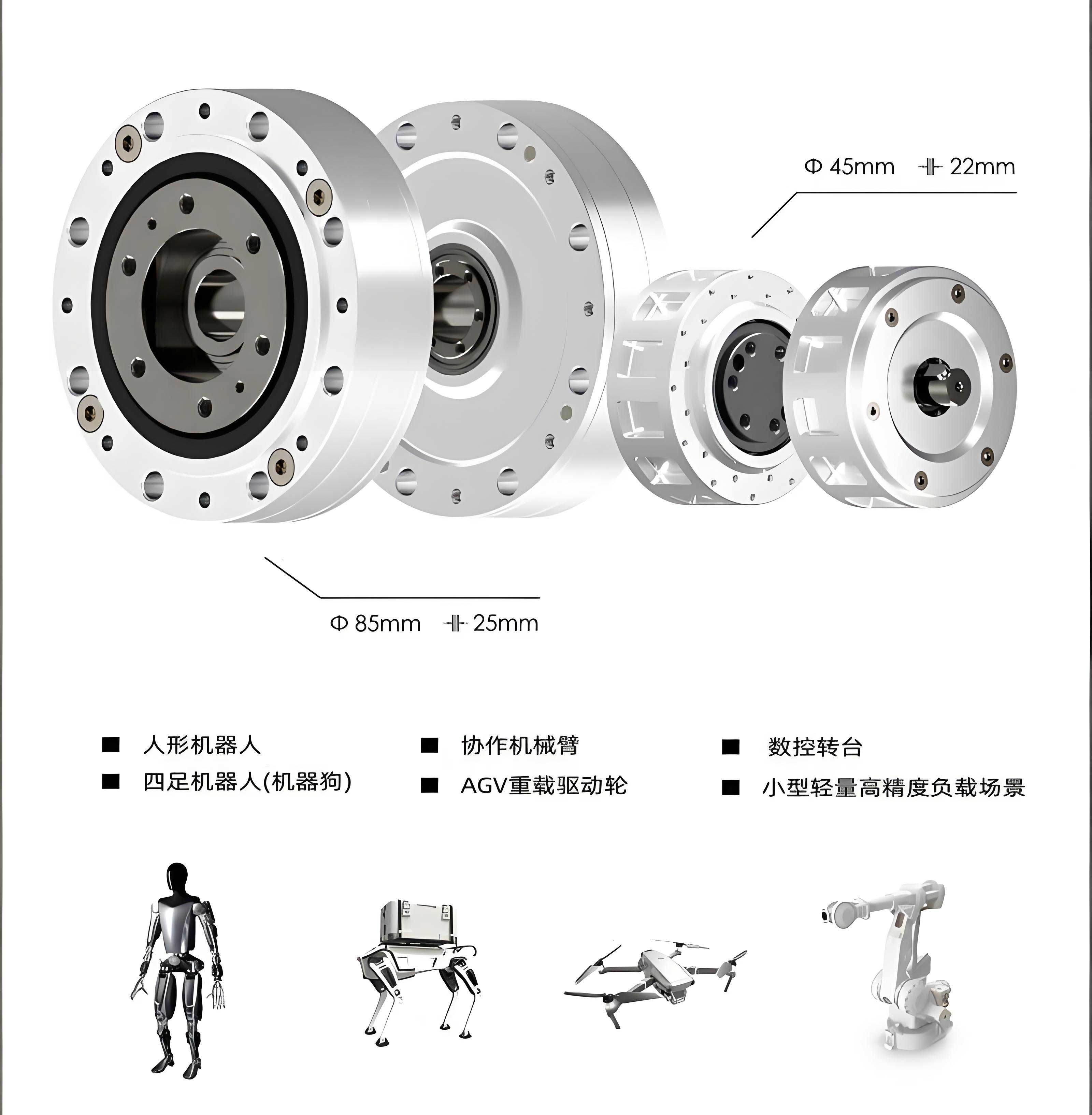
The RV reducer, renowned for its high reduction ratio, compactness, and torsional rigidity, operates on a two-stage reduction principle. The primary stage consists of a planetary gear train, where a sun gear meshes with multiple planetary gears, achieving the first level of speed reduction. The secondary, and most distinctive, stage is the cycloidal drive. Here, the planetary gears are rigidly connected to eccentric crankshafts. These crankshafts drive cycloid discs, which mesh with a stationary ring of needle rollers (the pinwheel). The rotation of the crankshafts causes an eccentric motion of the cycloid discs. This motion, constrained by the meshing with the pinwheel, is converted into a reduced rotational speed of the cycloid disc itself. An output flange, connected to the cycloid discs via pins, finally delivers the slow, high-torque output. This ingenious design is the source of the RV reducer’s advantageous characteristics.
Establishing the Dynamic Foundation: Mathematical Modeling
To effectively analyze and control transmission accuracy, a robust dynamic model of the RV reducer is indispensable. This model serves as the computational bridge between physical design parameters and system-level performance metrics. The modeling approach involves deriving equations of motion for each key component under the influence of internal forces, elastic deformations, and crucially, various error excitations.
To manage complexity, the model is built upon several justifiable simplifying assumptions:
- Bearings are treated as rigid supports.
- Gravitational forces on components are neglected.
- Friction in gear meshes is not considered.
- The system is perfectly aligned axially.
- Average equivalent stiffness values are used for similar connections.
- The input shaft rotates at a constant angular velocity.
- The deformation between a planetary gear and its crankshaft is congruent.
- A uniform damping coefficient is assumed for the system.
- Time-varying meshing stiffness in both gear stages is approximated by its average value over an engagement cycle.
The dynamic equilibrium equations for the core components are formulated considering their translational and rotational degrees of freedom. Let’s define the key coordinate systems and variables:
- $$m_s, m_p, m_b, m_{ca}$$: Masses of the sun gear, planetary gear, cycloid disc, and output carrier, respectively.
- $$J_s, J_p, J_b, J_{ca}$$: Moments of inertia of the sun gear, planetary gear, cycloid disc, and output carrier.
- $$x_i, y_i$$: Translational displacements of component i in the global coordinate plane.
- $$\theta_s, \theta_p, \theta_b, \theta_{ca}$$: Rotational angles of the sun gear, planetary gear, cycloid disc, and output carrier.
- $$R_{bp}, R_d$$: Base circle radius of the planetary gear and the distribution circle radius of the crankshafts.
- $$e$$: Eccentricity of the crankshaft.
- $$F_{ij}, C_{ij}$$: Elastic force and damping force components between components i and j.
- $$T_{out}$$: Output load torque.
The simplified dynamic equations for the planetary stage (sun and planetary gear) and the cycloidal stage can be represented. For the sun gear:
$$
m_s \ddot{x}_s + F_{sx} + (F_{1x} + C_{1x}) = 0
$$
$$
m_s \ddot{y}_s + F_{sy} + (F_{1y} + C_{1y}) = 0
$$
$$
J_s \ddot{\theta}_s = T_{in} – \sum (F_{1t} \cdot R_{bs})
$$
For a planetary gear (considering its revolution with the carrier):
$$
m_p (\ddot{x}_p – \dot{\theta}_{ca}^2 R_d \cos(\theta_{ca}+\phi) – \ddot{\theta}_{ca} R_d \sin(\theta_{ca}+\phi)) – (F_{1x}+C_{1x}) + (F_{2x}+C_{2x}) = 0
$$
$$
m_p (\ddot{y}_p – \dot{\theta}_{ca}^2 R_d \sin(\theta_{ca}+\phi) + \ddot{\theta}_{ca} R_d \cos(\theta_{ca}+\phi)) – (F_{1y}+C_{1y}) + (F_{2y}+C_{2y}) = 0
$$
$$
J_p \ddot{\theta}_p – (F_{1t} \cdot R_{bp}) – e \sum [ (F_{2ix}+C_{2ix})\sin(\theta_p+\psi_j) + (F_{2iy}+C_{2iy})\cos(\theta_p+\psi_j) ] = 0
$$
The forces $$F_{1}$$ and $$F_{2}$$ represent the sun-planet and planet-crankshaft interactions, respectively. The equations for the cycloid disc are more complex due to the eccentric motion and multi-tooth contact with the pinwheel. They involve terms for the relative acceleration of the disc center, centrifugal, and Coriolis effects. The general form for the cycloid disc dynamics in the rotating frame attached to the crankshaft can be expressed as:
$$
m_b[\ddot{\eta}_{dj}\cos(\gamma) – e\dot{\theta}_p^2\cos(\gamma) – e\ddot{\theta}_p\sin(\gamma) – 2\dot{\theta}_p\dot{\eta}_{dj}\sin(\gamma)] – F_{2jx} + \sum_{k=1}^{Z_p}(F_{cjk}+C_{cjk})\cos(\alpha_{jk}+\gamma)=0
$$
$$
m_b[\ddot{\eta}_{dj}\sin(\gamma) – e\dot{\theta}_p^2\sin(\gamma) + e\ddot{\theta}_p\cos(\gamma) + 2\dot{\theta}_p\dot{\eta}_{dj}\cos(\gamma)] + F_{2jy} + \sum_{k=1}^{Z_p}(F_{cjk}+C_{cjk})\sin(\alpha_{jk}+\gamma)=0
$$
$$
J_{bj}\ddot{\theta}_{dj} – \sum_{k=1}^{Z_p}(F_{cjk}+C_{cjk})R_{rw}\sin\alpha_{jk} – R_d[ (F_{2jy}+C_{2jy})\cos(\delta) – (F_{2jx}+C_{2jx})\sin(\delta) ] = 0
$$
where $$\eta_{dj}$$ is a relative displacement, $$\gamma = \theta_p + \psi_j$$, $$Z_p$$ is the number of pinwheel teeth, $$F_{cjk}$$ is the contact force with the k-th pin, $$\alpha_{jk}$$ is the contact angle, $$R_{rw}$$ is the radius of the rolling circle, and $$\delta$$ is a phase angle related to the crankshaft.
The system of equations for the entire RV reducer can be succinctly assembled into a matrix form, which is standard for multi-body dynamics:
$$
\mathbf{M}\ddot{\mathbf{X}} + \mathbf{C}\dot{\mathbf{X}} + \mathbf{K}\mathbf{X} = \mathbf{F}
$$
Here, $$\mathbf{M}$$, $$\mathbf{C}$$, and $$\mathbf{K}$$ are the global mass, damping, and stiffness matrices, respectively. $$\mathbf{X}$$ is the vector of generalized coordinates (all displacements and angles), and $$\mathbf{F}$$ is the vector of generalized forces, including the input torque and output load. This model becomes the essential “digital twin” for simulating the dynamic behavior of the RV reducer under the influence of design parameters and their inherent deviations.
Transmission Accuracy: The Key Performance Indicator
For precision applications like robotic joints, the transmission error is a paramount performance metric for the RV reducer. It quantifies the deviation between the expected and actual output position for a given input. In this analysis, transmission accuracy is defined by the dynamic transmission error (DTE), calculated at the output stage. The primary metric used is the difference between the ideal output carrier rotation and its actual simulated rotation over time.
$$
\Delta \theta(t) = \frac{\theta_s(t)}{i} – \theta_{ca}(t)
$$
where $$i$$ is the ideal reduction ratio of the RV reducer. The root-mean-square (RMS) or peak-to-peak value of $$\Delta \theta(t)$$ over an operational cycle serves as a scalar measure of transmission accuracy. The goal of tolerance design is to ensure that this measure remains within a specified allowable limit, the transmission accuracy tolerance $$T_A$$, despite manufacturing variations. For instance, a target might be set to reduce the peak-to-peak DTE from 40 arc-seconds to 20 arc-seconds.
| Performance Metric | Initial Benchmark | Design Target |
|---|---|---|
| Transmission Accuracy (Peak-to-Peak DTE) | 40 arc-seconds | ≤ 20 arc-seconds |
Performance Consistency Design: From System Target to Parameter Tolerances
The core contribution of this work lies in the systematic methodology for decomposing the system-level performance tolerance ($$T_A$$) into component-level parameter tolerances. This process, known as performance consistency design, involves three major steps.
Step 1: Identification and Screening of Critical Design Parameters
Not all design parameters of an RV reducer influence transmission accuracy equally. The first step is to conduct a global sensitivity analysis using the dynamic model. Parameters are perturbed within a small, realistic range, and the corresponding change in the DTE metric ($$\Delta \theta_{RMS}$$) is computed. The sensitivity coefficient $$S_i$$ for parameter $$p_i$$ can be defined as:
$$
S_i = \frac{\partial (\Delta \theta_{RMS})}{\partial p_i} \approx \frac{\Delta (\Delta \theta_{RMS})}{\Delta p_i}
$$
Parameters with high $$|S_i|$$ values have a strong influence on performance and are classified as “Critical-to-Quality” (CTQ) parameters for tolerance allocation. Based on prior research and dynamic analysis, the following parameters are typically identified as highly sensitive for the RV reducer:
- Pinwheel Tooth Profile Error ($$e_{p,prof}$$): Deviation from the ideal circular form of the pinwheel seat.
- Pinwheel Cumulative Pitch Error ($$e_{p,pitch}$$): Error in the angular positioning of the pins around the pinwheel.
- Cycloid Disc Tooth Profile Error ($$e_{c,prof}$$): Deviation from the ideal cycloidal profile of the disc.
- Cycloid Disc Cumulative Pitch Error ($$e_{c,pitch}$$): Error in the angular spacing of the cycloid disc teeth.
- Crankshaft Eccentricity Error ($$e_{cr}$$): Deviation of the actual eccentricity from its nominal design value.
- Clearance in the Crankshaft-Cycloid Bearing ($$\delta_{bearing}$$): Radial play in the bearing connecting the crankshaft throw to the cycloid disc.
These errors are often modeled as harmonic functions, e.g., $$e_{p,prof}(\theta_k) = A_{prof} \sin(2\theta_k + \phi)$$, where their amplitude becomes the sensitivity parameter.
| Critical Design Parameter (Error Source) | Symbol | Typical Formulation | Initial Nominal Value |
|---|---|---|---|
| Pinwheel Tooth Profile Error | $$e_{p,prof}$$ | $$A_{pp} \sin(2\theta_k)$$ | 0 μm |
| Pinwheel Cumulative Pitch Error | $$e_{p,pitch}$$ | $$A_{pc} \sin(2\theta_k)$$ | 0 arc-sec |
| Cycloid Disc Tooth Profile Error | $$e_{c,prof}$$ | $$A_{cp} \sin(2\theta_d)$$ | 0 μm |
| Cycloid Disc Cumulative Pitch Error | $$e_{c,pitch}$$ | $$A_{cc} \sin(2\theta_d)$$ | 0 arc-sec |
| Crankshaft Eccentricity Error | $$e_{cr}$$ | Constant offset | 0 μm |
| Crankshaft-Cycloid Bearing Clearance | $$\delta_{bearing}$$ | Constant radial gap | 0 μm |
Step 2: Sensitivity and Coupling Analysis
With the CTQ parameters identified, a more refined analysis quantifies not only their individual sensitivity but also potential coupling effects. A designed experiment (e.g., using Latin Hypercube Sampling) is conducted within the multi-dimensional parameter space. The dynamic model is run for each sample set, and the resulting DTE is recorded. Statistical analysis, such as Analysis of Variance (ANOVA), is then performed on the results. This yields a ranked list of parameters based on their contribution to the variance in DTE output.
| Rank | Design Parameter | Contribution to DTE Variance (%) | Remarks |
|---|---|---|---|
| 1 | Cycloid Disc Tooth Profile Error ($$A_{cp}$$) | ~35% | Highest sensitivity, direct contact geometry. |
| 2 | Crankshaft Eccentricity Error ($$e_{cr}$$) | ~25% | Directly affects the cycloid disc motion law. |
| 3 | Pinwheel Tooth Profile Error ($$A_{pp}$$) | ~20% | Counterpart contact surface to cycloid disc. |
| 4 | Bearing Clearance ($$\delta_{bearing}$$) | ~12% | Introduces non-linear backlash-type effects. |
| 5 | Cycloid Disc Pitch Error ($$A_{cc}$$) | ~5% | Less critical than profile form. |
| 6 | Pinwheel Pitch Error ($$A_{pc}$$) | ~3% | Least sensitive among the CTQ parameters. |
Step 3: Decomposition of System Tolerance to Parameter Tolerances
This is the optimization core. The goal is to find the allowable tolerance range ($$ \pm \Delta p_i $$) for each CTQ parameter such that the resulting DTE is guaranteed to stay within the system tolerance $$T_A$$ (e.g., 20 arc-seconds), even under worst-case or statistically likely combinations of these parameter deviations. A linearized approach near the nominal design point is often effective for initial allocation.
The relationship between DTE and parameters can be linearized as:
$$
\Delta \theta \approx \sum_{i=1}^{n} S_i \cdot \Delta p_i
$$
where $$S_i$$ is the sensitivity coefficient and $$\Delta p_i$$ is the deviation from nominal for the i-th parameter. To ensure the performance constraint, we require:
$$
\left| \sum_{i=1}^{n} S_i \cdot \Delta p_i \right| \leq T_A
$$
The challenge is that there are infinite combinations of $$\Delta p_i$$ that satisfy this inequality. The optimization seeks the combination that maximizes the manufacturability, often formulated as finding the largest permissible tolerance zones. A common method is the “Root Sum Square” (RSS) allocation for statistical tolerance analysis, assuming independent, normally distributed errors:
$$
T_A^2 \geq \sum_{i=1}^{n} (S_i^2 \cdot T_{p,i}^2)
$$
where $$T_{p,i}$$ is the tolerance allocated to parameter $$p_i$$. The individual tolerances can be allocated proportionally to the inverse of their sensitivity or cost factor $$c_i$$:
$$
T_{p,i} = \frac{T_A}{ |S_i| \sqrt{\sum_{j=1}^{n} (S_j^2 / c_j^2)}} \cdot \frac{1}{c_i}
$$
This assigns tighter tolerances to highly sensitive or cheap-to-tighten parameters, and looser tolerances to less sensitive or expensive ones.
For a more rigorous and optimal allocation, a formal optimization problem can be set up. The objective is to minimize a total cost function $$C_{total}$$ associated with achieving a given tolerance level (tighter tolerances generally cost more). The constraints ensure the dynamic performance is met.
$$
\begin{aligned}
& \underset{T_{p,1},…, T_{p,n}}{\text{minimize}}
& & C_{total} = \sum_{i=1}^{n} f_i(T_{p,i}) \\
& \text{subject to}
& & P(\Delta \theta_{RMS}(p_i + \Delta p_i) \leq T_A) \geq \eta \\
& & & T_{p,i}^{min} \leq T_{p,i} \leq T_{p,i}^{max}
\end{aligned}
$$
Here, $$f_i(T_{p,i})$$ is the cost-tolerance function for parameter i (often exponential or reciprocal), and $$\eta$$ is the desired confidence level (e.g., 99.7% for a 3-sigma process). This problem is solved using optimization algorithms like Genetic Algorithms (GA) or Sequential Quadratic Programming (SQP), with the dynamic model acting as the constraint evaluator.
| Design Parameter | Nominal Value | Initial (Tight) Tolerance | Optimized (Relaxed) Tolerance | Relaxation | Comment |
|---|---|---|---|---|---|
| Cycloid Disc Profile Error ($$A_{cp}$$) | 0 μm | ±3 μm | ±4.5 μm | +50% | High sensitivity limits relaxation. |
| Crankshaft Eccentricity ($$e_{cr}$$) | 1.5 mm | ±2 μm | ±1.8 μm | -10% | May need tightening to compensate for others. |
| Pinwheel Profile Error ($$A_{pp}$$) | 0 μm | ±3 μm | ±5.2 μm | +73% | Significant relaxation possible. |
| Bearing Clearance ($$\delta_{bearing}$$) | 0 μm | ±5 μm | ±8 μm | +60% | Commercial bearing grades become acceptable. |
| Cycloid Disc Pitch Error ($$A_{cc}$$) | 0 arc-sec | ±15 arc-sec | ±30 arc-sec | +100% | Low sensitivity allows major relaxation. |
| Pinwheel Pitch Error ($$A_{pc}$$) | 0 arc-sec | ±15 arc-sec | ±35 arc-sec | +133% | Greatest relaxation due to lowest sensitivity. |
Integrated Optimization Framework and Expected Outcomes
The proposed methodology integrates dynamics, sensitivity analysis, and tolerance optimization into a cohesive computer-aided engineering framework for the RV reducer. The workflow is as follows:
- Model Creation: Develop and validate the parameterized multi-body dynamic model of the RV reducer.
- Target Definition: Set the system-level transmission accuracy target ($$T_A$$).
- Screening: Perform a global sensitivity analysis to identify the shortlist of CTQ design parameters.
- Meta-modeling: Optionally, create a fast-running surrogate model (e.g., Response Surface Model, neural network) of the DTE as a function of the CTQ parameters to speed up optimization.
- Tolerance Optimization: Solve the tolerance allocation optimization problem (cost minimization or tolerance maximization) subject to the DTE constraint.
- Verification: Run Monte Carlo simulations using the dynamic model with parameters varying within their newly allocated optimal tolerances to statistically verify that the DTE target is met.
The primary outcome is a set of optimized, performance-guaranteed tolerance specifications for the manufacturing drawings. For the manufacturer, this translates directly into tangible benefits:
- Reduced Manufacturing Cost: Relaxing tolerances on less sensitive parameters (e.g., pitch errors) allows the use of standard or less precise machining processes.
- Improved Consistency: By focusing control efforts on the few highly sensitive parameters, overall product quality consistency is improved.
- Enhanced Competitiveness: The ability to produce an RV reducer that meets high-performance standards at a lower cost is a significant market advantage.
- Informed Design Trade-offs: The framework quantitatively shows the performance cost of relaxing any tolerance, enabling intelligent design decisions.
Conclusion and Forward Outlook
This detailed exploration underscores that mastering the performance of an RV reducer requires moving beyond deterministic design into the realm of variation-aware design. By constructing a high-fidelity dynamic model, we establish the essential causal link between microscopic geometric and assembly parameters and the macroscopic system behavior. The systematic application of sensitivity analysis and tolerance optimization algorithms allows us to decompose a system-level performance target—transmission accuracy—into a scientifically grounded set of component-level manufacturing tolerances.
The significance of this approach lies in its proactive nature. Instead of over-designing every component with prohibitively tight tolerances or engaging in costly post-production sorting, it enables the intelligent allocation of precision where it is dynamically necessary. This methodology directly addresses the core challenges in high-volume precision manufacturing of complex systems like the RV reducer: achieving consistent performance while controlling costs. Future work will involve extending the model to include thermal effects, non-linear stiffness from bearings and contacts, and applying robust design principles to make the RV reducer’s performance less sensitive to variations in the operating environment and load conditions.
| Optimization Scenario | DTE (arc-sec, pk-pk) | Estimated Relative Manufacturing Cost | Key Tolerance Change | Trade-off Insight |
|---|---|---|---|---|
| Baseline (All Tight Tolerances) | 15 | 1.00 (Reference) | – | Over-engineered, high cost. |
| Cost-Optimized (Target DTE ≤ 20) | 19.5 | 0.65 | Pitch errors greatly relaxed. | 35% cost saving for minimal performance loss. |
| Performance-Optimized (Min DTE) | 10 | 1.40 | Profile & eccentricity tolerances halved. | 33% performance gain at 40% cost increase. |
| Balanced Design | 17 | 0.80 | Moderate relaxation across all parameters. | Best practical compromise for mass production. |