
The deep integration of information technology and manufacturing is spearheading a transformation in production methods. The advancement of industrial robotics is pivotal to this smart manufacturing revolution. The high-precision reducer stands as a core component of industrial robots, largely determining their transmission accuracy. To precisely execute motion transfer from the motor and guarantee transmission precision, these reducers demand exceptionally high standards in both manufacturing and assembly accuracy. Assembly is the final, critical process that determines the quality of a precision reducer.
The RV reducer, as a two-stage high-precision speed reduction mechanism, is characterized by its compact size, intricate structure, and multitude of components. To achieve high transmission accuracy, the transmission error of an RV reducer is required to be controlled within 1 arc-minute. Consequently, the assembly clearance must be maintained within a few micrometers, a condition that traditional assembly methods often fail to meet consistently. Current research on selective assembly technology for mechanical products is extensive. Early work solved the hole-and-shaft matching problem using a convex loss function, targeting an optimal clearance of 12 μm. Other studies have addressed selection issues in assemblies like crankshaft connecting rods and pistons & cylinders, employing methods such as Genetic Algorithms (GA), Signal-to-Noise Ratio (SNR)-based loss functions, and Particle Swarm Optimization (PSO), often focusing on minimizing surplus parts or assembly gap fluctuation. Many of these approaches require part grouping based on dimensional distributions. Specific research on the RV reducer has applied bipartite graph maximum matching theory to optimize the pairing between the planetary carrier and the cycloid gear set.
However, comprehensive research on the selective assembly for the secondary transmission stage of the RV reducer, which significantly impacts overall transmission accuracy, remains limited. This article first analyzes the fundamental structure and transmission principle of the RV reducer, along with the factors affecting its transmission accuracy. It then proposes two critical fitting relationships specifically for the secondary transmission mechanism. To simultaneously improve the assembly qualification rate and the fitting precision, a multi-objective selective assembly model is constructed. Finally, the Non-dominated Sorting Genetic Algorithm II (NSGA-II) is introduced to search for the optimal solution, achieving the goals of optimized qualification rate and precision, thereby solving the selective assembly problem for the secondary transmission stage.
Establishment of the Selective Assembly Mathematical Model
Basic Structure and Transmission Principle of the RV Reducer
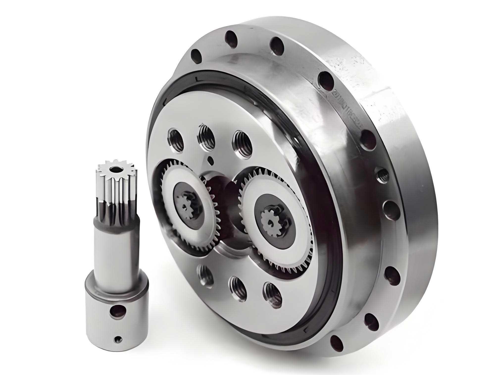
The RV reducer incorporates two stages of精密传动机构: a planetary gear stage and a cycloidal pin-wheel stage. Its main components include the input shaft, sun gear, planet gears, crankshafts, needle bearings, cycloid discs, pins (or needle pins), and the pin housing (pin wheel). During operation, the input shaft gear drives the planet gears, accomplishing the first stage of speed reduction. In the secondary stage, the crankshaft, fixed to the planet gear, transmits motion to the cycloid disc. The eccentric section of the crankshaft, via needle bearings, causes the cycloid disc to rotate about its own axis while simultaneously performing an eccentric revolution around the center of the pin housing. With the pin housing fixed, the motion is output through the planet carrier.
The primary factors affecting the transmission accuracy of the RV reducer are part machining errors and assembly errors. Errors in the secondary transmission stage have a more direct and pronounced impact on the output accuracy compared to those in the primary stage, which are scaled down by the reduction ratio before affecting the output.
Establishment of Fitting Relationships
Excessive clearance between components during assembly can cause transient output interruption, leading to angular error in the output shaft and increased transmission error. The transmission interface between the eccentric part of the crankshaft and the crank holes of the cycloid discs constitutes the input of the secondary stage, where bearing clearance exists post-assembly. To ensure proper meshing between the cycloid discs and the housing pins while maintaining adequate lubrication, this crankshaft bearing clearance must be controlled within a specific range. Within the cycloidal drive, numerous error terms affect transmission accuracy. Significant contributors include errors in the pin center circle radius, pin radius errors, and the clearance between pins and their housing bores. These errors manifest in the assembly clearances. To enhance transmission accuracy, assembly dimension chains can be established to minimize the impact of these error terms.
To control the crankshaft bearing clearance, the first assembly dimension chain (Fitting 1) is established. Here, $D_p$ is the needle bearing roller diameter, $D_h$ is the diameter of the cycloid disc’s crank hole, $D_z$ is the diameter of the crankshaft’s eccentric section, and $A_1$ is the resulting clearance, serving as the closing link of Fitting 1.
$$A_1 = D_h – D_z – 2 \times D_p$$
Considering the eccentricity and error factors in the cycloidal stage, a second fitting relationship is proposed. This involves the pin housing’s root diameter $l_s$, the pin diameter $l_p$, and the over-pins measurement $l_d$ obtained using a gauge pin of diameter $l_b = 5.953 \text{ mm}$. The closing link for Fitting 2 is defined as $A_2$.
$$A_2 = l_s – l_d – 2 \times l_p$$
The magnitude of the closing link directly influences the fitting quality. Each closing link must be constrained within a specified tolerance range.
$$l_{i,j} \leq A_{i,j} \leq u_{i,j}$$
where $l_{i,j}$ is the lower limit and $u_{i,j}$ is the upper limit for the closing link. $A_{i,j}$ represents the actual dimension, with $i$ denoting the $i$-th assembly set and $j$ denoting the $j$-th dimension chain within that set.
Evaluation Criteria
Fitting quality and part quality are key determinants of an assembly’s final quality. While part quality is fixed during design and manufacturing, fitting quality is reflected in the assembly precision. Since selective assembly involves multiple sets, the assembly qualification rate is another critical evaluation metric.
Assembly Qualification Rate ($\eta$)
An RV reducer product is deemed qualified if all its closing links satisfy their respective constraint conditions. The qualification rate for a given selection scheme $t$ is defined as:
$$\eta_t = \frac{x_t}{X_t} \times 100\%$$
where $x_t$ is the number of qualified products in scheme $t$, and $X_t$ is the total number of assembly sets in scheme $t$.
Fitting Precision ($f$)
A primary goal in RV reducer assembly is ensuring fitting precision, which is a necessary condition for product qualification. For superior performance, assembly clearances should approach their optimal target values. For a preliminary scheme containing $n$ assembly sets, each with $j$ dimension chains, fitting precision is optimized by minimizing the deviation of the actual closing link value from its target. To formulate this as a maximization problem, fitting precision is defined as:
$$f = \frac{1}{n} \sum_{i=1}^{n} \left( 1 – \frac{|A_{i,j} – g_{i,j}|}{\Delta_{i,j}} \right)$$
where $A_{i,j}$, $g_{i,j}$, and $\Delta_{i,j}$ are the actual dimension, target dimension, and tolerance range, respectively, for the $j$-th closing link of the $i$-th assembly set.
Multi-objective Selective Assembly Mathematical Model
The dimensional data for the RV reducer parts involved in the selection can be represented in a matrix $\theta$, where each row corresponds to the dimensional data of the parts for one assembly set, and $n$ is the number of sets.
$$
\theta = \begin{pmatrix}
a_{11} & \ldots & a_{16} \\
\vdots & \ddots & \vdots \\
a_{n1} & \ldots & a_{n6}
\end{pmatrix}
$$
The cycloidal stage involves two cycloid discs, leading to four assembly dimension chains from the two fitting relationships. Both the qualification rate and fitting precision jointly determine the quality of an optimization scheme. Therefore, the multi-objective selective assembly mathematical model for the secondary stage of the RV reducer is established as:
$$
\begin{aligned}
& \text{M} = \quad \max \quad [ \eta(\theta), \quad f(\theta) ] \\
& \text{subject to:} \\
& D_h^1 – D_z – 2 \times D_p = A_1^1 \in [l_1, u_1] \\
& D_h^2 – D_z – 2 \times D_p = A_1^2 \in [l_1, u_1] \\
& l_s – l_d^1 – 2 \times l_p = A_2^1 \in [l_2, u_2] \\
& l_s – l_d^2 – 2 \times l_p = A_2^2 \in [l_2, u_2]
\end{aligned}
$$
Part Selective Assembly Design Based on NSGA-II
Manual selective assembly methods suffer from high randomness in part selection, where the assembly accuracy of the RV reducer depends heavily on its machining precision. This often leads to suboptimal assembly accuracy, low qualification rates, and high trial-and-error costs. Employing an intelligent algorithm to search the solution space for optimal schemes can simultaneously ensure efficiency, accuracy, and qualification rate. Among various multi-objective evolutionary algorithms, NSGA-II (Non-dominated Sorting Genetic Algorithm II) is renowned for its operational efficiency, stability, and convergence, making it well-suited for solving this problem.
Encoding Scheme
Encoding maps solution data from the search space for genetic evolution. The choice of encoding significantly impacts the computational results. Given the large number of parts involved in the selection for the RV reducer, a position-based matrix real-number encoding scheme is adopted. Each gene in the chromosome corresponds to the position of a part in the dimensional data matrix $\theta$. A chromosome is represented as a matrix $s$:
$$
s = \begin{pmatrix}
\beta_{11} & \ldots & \beta_{16} \\
\vdots & \ddots & \vdots \\
\beta_{n1} & \ldots & \beta_{n6}
\end{pmatrix}
$$
where $\beta_{ij}$ represents the position/index of the part for the $j$-th component in the $i$-th assembly set within the pooled inventory.
Multi-objective Optimization Based on NSGA-II
Dominance Relation in Objective Space
In a multi-objective problem with objective function vector $[f_1, f_2, …, f_l]$, for any two individuals $s_1$ and $s_2$ in the population, if $f_i(s_1) \geq f_i(s_2)$ for all $i \in [1, 2, …, l]$, and there exists at least one $i$ such that $f_i(s_1) > f_i(s_2)$, then individual $s_1$ is said to dominate individual $s_2$.
Fitness
Fitness is determined by both non-domination rank and crowding distance, which together define an individual’s priority. During fast non-dominated sorting, individuals are categorized into different fronts (ranks). A lower front number indicates a lower level of domination and a superior individual. Crowding distance $cd$ measures the density of individuals around a given individual within the same front, promoting diversity. For an individual $s[i,k]$ (the $i$-th individual when sorted by the $k$-th objective), the crowding distance is calculated as:
$$cd(s[i,k]) = \frac{f(s[i-1,k]) – f(s[i+1,k])}{f_{max} – f_{min}}$$
where $f_{max}$ and $f_{min}$ are the maximum and minimum values of the $k$-th objective function in that front.
Algorithm Workflow
1. Population Initialization: The initial population is generated using non-repetitive random permutation sampling for each column (part type). The population size is controlled based on the number of assembly sets. The iteration counter is set to $i = 0$.
2. Non-dominated Sorting and Crowding Distance Calculation: The dominance relations between individuals are determined by evaluating the objective functions. For each individual $s_i$, the number of individuals dominating it ($s_n$) and the number of individuals it dominates ($s_p$) are computed. Individuals are then sorted into non-dominated fronts based on these counts. The crowding distance for each individual within a front is calculated using the formula above and summed across all objectives.
3. Tournament Selection: This operator selects parent individuals for crossover and mutation based on their front rank ($i_{rank}$) and crowding distance ($i_{distance}$). Two distinct individuals are randomly chosen from the population. The individual with the better (lower) front rank is selected. If ranks are equal, the individual with the larger crowding distance is preferred.
4. Crossover and Mutation Operators: A partially mapped crossover (PMX) operator is employed. Two parent individuals are randomly selected. A crossover segment (with the same column indices for all rows) is defined by random start and end points. Genes within this segment are swapped between the two parents, column by column. This often creates invalid chromosomes with duplicate part indices outside the crossover segment. A mapping relationship is established from the genes in the crossover segment of one parent to the corresponding genes from the other parent. Genes outside the crossover segment that conflict with the new genes inside are repaired using this mapping. This process yields two valid offspring chromosomes.
For mutation, a swap mutation operator is used. Within a selected chromosome, two gene positions (within the same column) are randomly chosen and their values are exchanged. This enhances the local search capability of the algorithm.
5. Elitist Selection: Before elitist selection, the offspring population is combined with the parent population to preserve elite individuals. Selection for the next generation is then performed based on front rank and crowding distance, prioritizing individuals from better fronts until the population size is reached.
6. Termination Condition: The process iterates until a predefined maximum generation count $g$ is reached ($i \geq g$), at which point the optimal set of solutions (Pareto front) is output.
Analysis of Selective Assembly Results Based on NSGA-II
The selective assembly process was applied to the secondary reduction stage of an RV-20E-150BX model reducer. The parts involved included the crankshaft, needle bearings, cycloid discs (disc A and disc B, treated as separate entities due to high manufacturing variability), pins, and the pin housing. For a batch of $n$ RV reducer sets, the solution space has $n^6$ possibilities, which is vast. This study focused on selecting parts for 30 assembly sets, resulting in a sample space of $30^6 = 7.29 \times 10^8$ possible combinations. A subset of the dimensional data for the RV reducer parts is shown in the table below.
| Part Data ID | $D_h^1$ (mm) | $D_h^2$ (mm) | $D_p$ (mm) | $l_p$ (mm) | $D_z$ (mm) | $l_d^1$ (mm) | $l_d^2$ (mm) | $l_s$ (mm) |
|---|---|---|---|---|---|---|---|---|
| 1 | 25.999 | 25.999 | 2.9995 | 4.9985 | 20.0001 | 96.242 | 96.241 | 108.003 |
| 2 | 25.998 | 25.998 | 2.9985 | 4.993 | 20.0002 | 96.245 | 96.247 | 107.995 |
| 3 | 25.999 | 25.999 | 2.9995 | 4.997 | 20.0000 | 96.241 | 96.244 | 107.9997 |
| … | … | … | … | … | … | … | … | … |
| 15 | 26.000 | 26.000 | 2.9995 | 4.9985 | 20.0001 | 96.249 | 96.250 | 108.0049 |
In the designed assembly dimension chains, the tolerance for the closing link of Fitting 1 was $A_1 = 0^{+0.003}_{-0.001}$ mm, and for Fitting 2 it was $A_2 = 1.763^{+0.006}_{-0.002}$ mm. The NSGA-II parameters were set as follows: crossover probability $P_c = 0.6$, mutation probability $P_m = 0.01$, population size = 100, chromosome length = 30. Multiple optimization runs indicated the algorithm converged after approximately 200 generations.
A portion of the optimal selective assembly results and the corresponding closing link dimensions are shown in the following tables.
| Assembly Set ID | Cycloid A ID | Cycloid B ID | Crankshaft ID | Needle Bearing ID | Pin Housing ID | Pin ID | Qualified? |
|---|---|---|---|---|---|---|---|
| 1 | 20 | 30 | 29 | 24 | 22 | 25 | Yes |
| 2 | 6 | 5 | 6 | 30 | 21 | 27 | Yes |
| 3 | 10 | 26 | 7 | 3 | 17 | 3 | Yes |
| … | … | … | … | … | … | … | … |
| 13 | 5 | 28 | 24 | 28 | 5 | 9 | No |
| 14 | 24 | 14 | 26 | 27 | 3 | 13 | Yes |
| 15 | 14 | 13 | 18 | 1 | 7 | 16 | Yes |
| Set ID | $A_1^1$ (mm) | Qualified? | $A_1^2$ (mm) | Qualified? | $A_2^1$ (mm) | Qualified? | $A_2^2$ (mm) | Qualified? |
|---|---|---|---|---|---|---|---|---|
| 1 | 0.0018 | Yes | 0.0018 | Yes | 1.7643 | Yes | 1.7653 | Yes |
| 2 | 0.0019 | Yes | 0.0009 | Yes | 1.7632 | Yes | 1.7652 | Yes |
| 3 | 0.0000 | Yes | 0.0000 | Yes | 1.7660 | Yes | 1.7650 | Yes |
| … | … | … | … | … | … | … | … | … |
| 13 | 0.0009 | Yes | 0.0009 | Yes | 1.7530 | No | 1.7520 | No |
The comparison between the proposed method and traditional manual selection is summarized in the table below. The NSGA-II-based optimization method demonstrates a substantial improvement in both key performance indicators for the RV reducer assembly.
| Selection Method | Assembly Qualification Rate | Fitting Precision ($f$) |
|---|---|---|
| Proposed NSGA-II Method | 96.67% | 3.4458 |
| Traditional Manual Method | 56.67% | 2.8225 |
Conclusion
The RV reducer requires high transmission accuracy, imposing stringent demands on assembly precision. The secondary cycloidal planetary transmission stage has the most significant impact on the overall assembly accuracy of the RV reducer. To ensure the assembly accuracy meets requirements, this study analyzed the transmission principle and structural characteristics of the RV reducer and proposed two fitting relationships for the crankshaft eccentric section and the cycloidal-pin transmission stage to minimize key error terms. Due to the low efficiency and inconsistent precision of traditional selective assembly methods, this paper established a multi-objective selective assembly mathematical model for the secondary stage of the RV reducer, using both assembly qualification rate and fitting precision as evaluation criteria.
The NSGA-II algorithm was employed to find the optimal assembly scheme. Considering the large number of parts involved, a position-based matrix real-number encoding scheme was utilized alongside a partially mapped crossover operator, which provided robust global search capabilities. Compared to the traditional manual method, the proposed approach achieved a dramatic increase in the assembly qualification rate and a significant improvement in fitting precision for the RV reducer. This method effectively solves the selective assembly problem for the critical secondary transmission stage of the RV reducer, offering a practical and efficient solution for high-precision assembly in industrial manufacturing.