
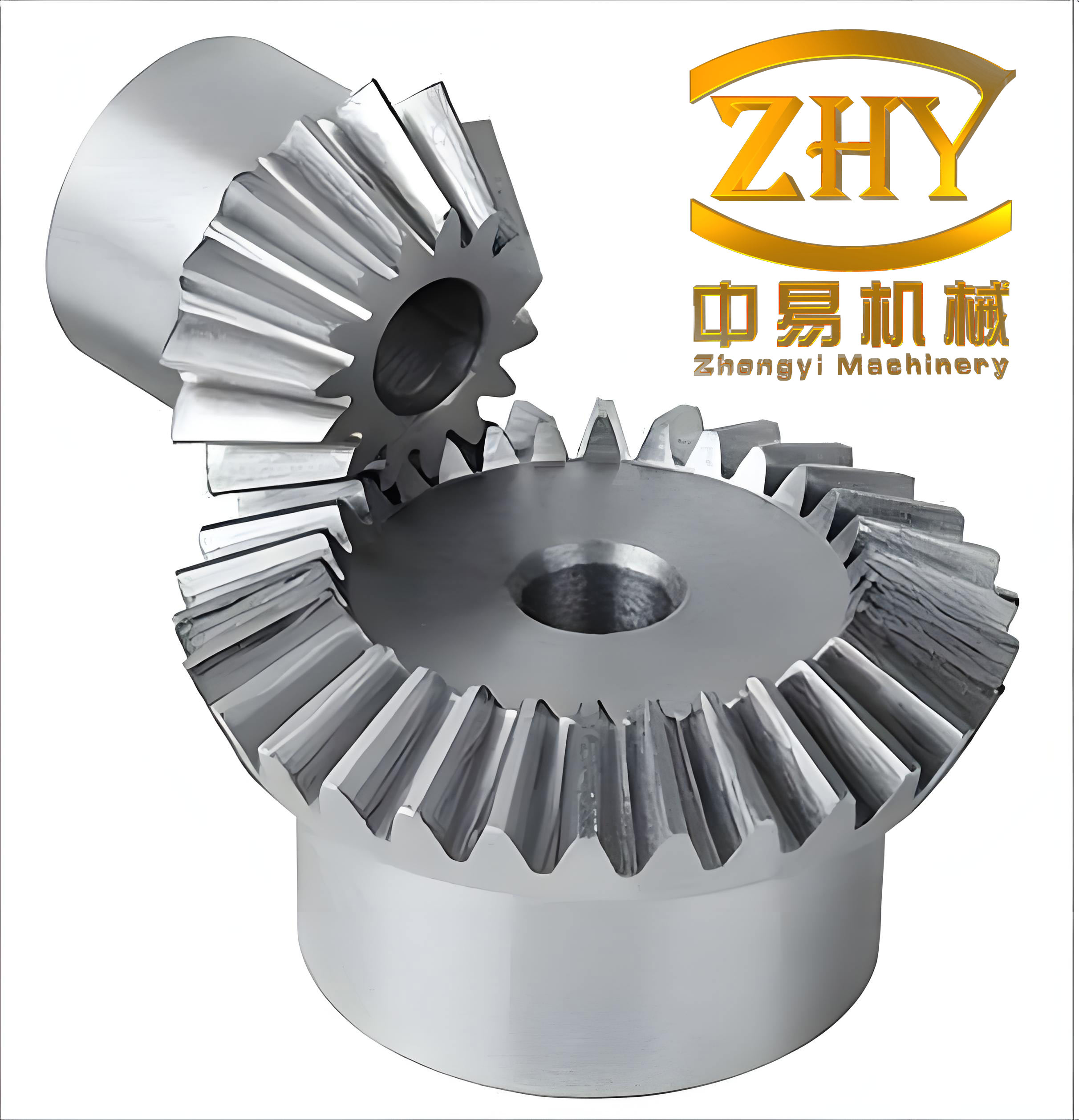
In this article, I will delve into the detailed analysis of tooth surface curvature radius and velocity for straight bevel gears. Straight bevel gears are a critical component in intersecting shaft transmissions, widely used in aerospace auxiliary power transmission and various industrial applications. The curvature radius of the tooth surface at the meshing point is a fundamental parameter that directly influences the meshing characteristics and transmission performance of gears. It serves as essential data for analyzing elastohydrodynamic (EHD) conditions and calculating contact stresses. Moreover, the relative rolling and sliding between meshing tooth surfaces are the driving forces for forming EHD oil films. Therefore, analyzing tooth surface velocity, especially in the rolling direction, is crucial for EHD lubrication analysis. Based on the generating principle of straight bevel gears, I will derive expressions for the tooth surface curvature radius and the composite curvature radius, comparing them with results from the equivalent gear method. Additionally, through numerical computation of tooth surface coordinates, I will analyze the velocity of points on the tooth surface, providing a foundation for precise EHD analysis and contact stress distribution under EHD conditions.
The geometry of straight bevel gears is complex due to their conical shape. The tooth surface is generated by a planar generating gear, and understanding the relationship between the generating surface and the generated tooth surface is key to deriving curvature properties. Let me start by outlining the coordinate systems and geometric model used in the analysis.
Consider the generating process of a straight bevel gear. A planar generating gear with a pitch cone angle \(\delta_g\) engages with the workpiece gear with pitch cone angle \(\delta_1\). The generating plane \(\Sigma_g\) is fixed to the generating gear. During cutting, the generating gear rolls purely on the pitch cone of the workpiece, enveloping the tooth surface \(\Sigma_1\). Similarly, the mating gear tooth surface \(\Sigma_2\) is generated. The coordinate systems are defined as follows: a fixed coordinate system \(O-xyz\) with the z-axis coinciding with the instantaneous meshing axis \(OP\). The generating gear coordinate system \(O_g-x_g y_g z_g\) and the workpiece coordinate system \(O_1-x_1 y_1 z_1\) are attached to their respective components.
Using module \(m\) and angle \(\beta\) as parameters, in the \(O_g-x_g y_g z_g\) system, the equation of the generating plane \(\Sigma_g\) is:
$$z_g = -x_g \tan \alpha \sin \beta + y_g \tan \alpha \cos \beta$$
where \(\alpha\) is the pressure angle. The unit normal vector to the plane is:
$$\mathbf{n}_g = \left( \frac{\tan \alpha \sin \beta}{\sqrt{1+\tan^2 \alpha}}, -\frac{\tan \alpha \cos \beta}{\sqrt{1+\tan^2 \alpha}}, \frac{1}{\sqrt{1+\tan^2 \alpha}} \right)^T$$
Transforming to the fixed coordinate system \(O-xyz\), the equation of the generating plane and its unit normal become:
$$\mathbf{r}_g = \begin{pmatrix} R \cos \phi \\ R \sin \phi \\ -R \tan \alpha \sin(\beta – \phi) \end{pmatrix}, \quad \mathbf{n} = \begin{pmatrix} \tan \alpha \sin \beta \cos \phi – \tan \alpha \cos \beta \sin \phi \\ \tan \alpha \sin \beta \sin \phi + \tan \alpha \cos \beta \cos \phi \\ 1 \end{pmatrix} \frac{1}{\sqrt{1+\tan^2 \alpha}}$$
Here, \(R\) is the cone distance, and \(\phi\) is the rotation angle of the generating gear. The meshing condition, derived from the common normal intersecting the meshing axis, is:
$$\phi = \beta – \arctan\left( \frac{\tan \alpha \sin \beta}{\tan \alpha \cos \beta + \cot \delta_1} \right)$$
For straight bevel gears, the instantaneous contact line always passes through the cone apex. The tooth surface is a ruled surface with one principal direction along the generatrix, corresponding to zero curvature. The other principal direction, perpendicular to the contact line, is of interest. Let \(\mathbf{e}\) be the unit vector in this direction on the generating surface. Since the generating surface is a plane, its curvature \(\kappa_g = 0\).
Denote the angular velocities of the generating gear, gear 1, and gear 2 as \(\boldsymbol{\omega}_g\), \(\boldsymbol{\omega}_1\), and \(\boldsymbol{\omega}_2\), respectively. Assuming \(\omega_g = 1\), the relative angular velocities are:
$$\boldsymbol{\omega}_{g1} = \boldsymbol{\omega}_g – \boldsymbol{\omega}_1 = \begin{pmatrix} 0 \\ 0 \\ 1 – \omega_1 \end{pmatrix}, \quad \boldsymbol{\omega}_{g2} = \boldsymbol{\omega}_g – \boldsymbol{\omega}_2 = \begin{pmatrix} 0 \\ 0 \\ 1 – \omega_2 \end{pmatrix}$$
The angular velocities are along the z-axis direction. The relative velocity of the contact point on the generating surface is:
$$\mathbf{v}_{g1} = \boldsymbol{\omega}_{g1} \times \mathbf{r}_g$$
After calculations, the curvature of the generated tooth surface \(\Sigma_1\) in the direction \(\mathbf{e}\) is given by:
$$\kappa_1 = \frac{ \left( \boldsymbol{\omega}_{g1} \times \mathbf{n} \right) \cdot \left( \mathbf{v}_{g1} \times \mathbf{e} \right) }{ \left( \mathbf{v}_{g1} \cdot \mathbf{e} \right)^2 }$$
Substituting the expressions for \(\mathbf{r}_g\), \(\mathbf{n}\), and \(\mathbf{e}\), we obtain:
$$\kappa_1 = \frac{ \sin \delta_1 \left( \cos \alpha \sin \beta \cos \phi – \cos \alpha \cos \beta \sin \phi \right) }{ R \left( \sin \alpha \sin \beta \cos \phi – \sin \alpha \cos \beta \sin \phi + \cos \delta_1 \right)^2 }$$
Similarly, for gear 2, the curvature \(\kappa_2\) can be derived. The composite curvature radius \(\rho_c\) for the meshing pair is defined as:
$$\frac{1}{\rho_c} = \frac{1}{\rho_1} + \frac{1}{\rho_2}$$
where \(\rho_1 = 1/\kappa_1\) and \(\rho_2 = 1/\kappa_2\) are the curvature radii of the tooth surfaces. For straight bevel gears, the expressions simplify. At the pitch point (\(\phi = 0\)), the curvature radii are:
$$\rho_1 = \frac{R \sin \delta_1}{\cos \alpha \sin \beta}, \quad \rho_2 = \frac{R \sin \delta_2}{\cos \alpha \sin \beta}$$
Thus, the composite curvature radius at the pitch point is:
$$\rho_c = \frac{R \sin \delta_1 \sin \delta_2}{\cos \alpha \sin \beta (\sin \delta_1 + \sin \delta_2)}$$
For orthogonal straight bevel gears (\(\delta_1 + \delta_2 = 90^\circ\)), this reduces to:
$$\rho_c = \frac{R \sin \delta_1 \sin \delta_2}{\cos \alpha \sin \beta}$$
In standard straight bevel gear design, the module at the back cone distance \(R\) is \(m_R = R / (z_1 \cos \delta_1)\), where \(z_1\) is the number of teeth on gear 1. Substituting, we get:
$$\rho_c = \frac{m_R z_1 \sin \delta_1 \sin \delta_2}{\cos \alpha \sin \beta \cos \delta_1}$$
This formula provides the composite curvature radius for straight bevel gears at any cone distance \(R\) and meshing position \(\phi\). To illustrate the variations, let me discuss the influencing factors.
The composite curvature radius \(\rho_c\) is proportional to the cone distance \(R\). Therefore, along the tooth width, \(\rho_c\) is largest at the heel (large end) and smallest at the toe (small end). Moreover, \(\rho_c\) varies with the meshing position \(\phi\). Taking the derivative with respect to \(\phi\), we find that \(\rho_c\) reaches an extreme value at the pitch point (\(\phi = 0\)). Specifically, for orthogonal gears, \(\rho_c\) is minimum at the pitch point and increases on both sides. This behavior is similar to spur gears but with conical geometry effects.
Another factor is the shaft angle. For a given pressure angle and module, \(\rho_c\) changes with the pitch cone angles \(\delta_1\) and \(\delta_2\). The maximum \(\rho_c\) occurs when \(\delta_1 = \delta_2 = 45^\circ\) (i.e., gear ratio \(i = 1\)), and it decreases symmetrically as the angles diverge.
In traditional strength calculations, the equivalent spur gear method is often used. The composite curvature radius from this method for straight bevel gears at the pitch point is:
$$\rho_{c,eq} = \frac{m_m z_{v1} \sin \alpha}{2} \cdot \frac{i}{i+1}$$
where \(m_m\) is the module at the mid-face width, \(z_{v1}\) is the virtual number of teeth, and \(i\) is the gear ratio. Comparing with our derived formula, the equivalent method only yields accurate results at the mid-face width and pitch point. Elsewhere, it introduces approximations. Therefore, for precise EHD analysis, the derived curvature expressions are essential.
Now, let’s move to velocity analysis. The velocity of points on the tooth surface is crucial for determining rolling and sliding components. Based on the generating principle, the tooth surface \(\Sigma_1\) can be parameterized by \(R\) and \(\phi\). In the coordinate system \(O-xyz\), the position vector \(\mathbf{r}_1\) and unit normal \(\mathbf{n}_1\) are functions of \(R\) and \(\phi\). The instantaneous contact line direction is along the generatrix, denoted by vector \(\mathbf{t}_1\). The tooth profile direction, perpendicular to the contact line, is denoted by \(\mathbf{s}_1\). These vectors satisfy:
$$\mathbf{t}_1 \cdot \mathbf{n}_1 = 0, \quad \mathbf{s}_1 \cdot \mathbf{n}_1 = 0, \quad \mathbf{t}_1 \cdot \mathbf{s}_1 = 0$$
When the coordinate system rotates with angular velocity \(\boldsymbol{\omega}_1\), the velocity of a point on the tooth surface is:
$$\mathbf{v}_1 = \boldsymbol{\omega}_1 \times \mathbf{r}_1$$
Since \(O-xyz\) is fixed to gear 1, this represents the absolute velocity. The velocity component in the rolling direction (along \(\mathbf{s}_1\)) is:
$$v_{1s} = \mathbf{v}_1 \cdot \mathbf{s}_1$$
Similarly, for gear 2, the velocity \(v_{2s}\) can be computed. The relative sliding velocity is:
$$v_s = |v_{1s} – v_{2s}|$$
Note that the actual directions depend on the driving and driven gears. If calculated velocities have the same sign, the actual directions are opposite, and vice versa.
For straight bevel gears, the velocity \(\mathbf{v}_1\) has no component in the tooth width direction, meaning there is no relative motion along the generatrix. This simplifies the analysis. The velocity magnitude is linear along the contact line, as \(\mathbf{r}_1\) is linear in \(R\). Thus, by computing velocities at the heel and toe, we can interpolate for other points.
To demonstrate, I present a numerical example. Consider a standard straight bevel gear pair with parameters: module \(m = 5 \, \text{mm}\), number of teeth \(z_1 = 20\), \(z_2 = 40\), pressure angle \(\alpha = 20^\circ\), shaft angle \(\Sigma = 90^\circ\), and face width \(b = 30 \, \text{mm}\). The pitch cone angles are \(\delta_1 = \arctan(z_1/z_2) = 26.565^\circ\) and \(\delta_2 = 63.435^\circ\). Assume angular velocity \(\omega_1 = 100 \, \text{rad/s}\) and \(\omega_2 = \omega_1 / i = 50 \, \text{rad/s}\), where \(i = z_2/z_1 = 2\).
I compute the curvature radii and velocities at the heel (\(R = R_{\text{max}}\)) for various meshing positions \(\phi\). The results are summarized in the following tables.
| Meshing Position \(\phi\) (degrees) | \(\rho_1\) (mm) | \(\rho_2\) (mm) | \(\rho_c\) (mm) |
|---|---|---|---|
| -30 | 45.2 | 90.4 | 30.1 |
| -20 | 42.8 | 85.6 | 28.5 |
| -10 | 40.5 | 81.0 | 27.0 |
| 0 (pitch point) | 38.2 | 76.4 | 25.5 |
| 10 | 40.5 | 81.0 | 27.0 |
| 20 | 42.8 | 85.6 | 28.5 |
| 30 | 45.2 | 90.4 | 30.1 |
Table 1 shows that \(\rho_c\) is minimum at the pitch point, as expected. The values are symmetric about \(\phi = 0\), reflecting the gear geometry.
| Meshing Position \(\phi\) (degrees) | \(v_{1s}\) (m/s) | \(v_{2s}\) (m/s) | Relative Sliding \(v_s\) (m/s) |
|---|---|---|---|
| -30 | 2.15 | -1.08 | 3.23 |
| -20 | 1.98 | -0.99 | 2.97 |
| -10 | 1.82 | -0.91 | 2.73 |
| 0 (pitch point) | 1.65 | -0.83 | 2.48 |
| 10 | 1.82 | -0.91 | 2.73 |
| 20 | 1.98 | -0.99 | 2.97 |
| 30 | 2.15 | -1.08 | 3.23 |
In Table 2, the velocities are calculated at the heel. The negative signs for \(v_{2s}\) indicate opposite direction to \(v_{1s}\). The relative sliding velocity is zero only at the pitch point in theory, but due to geometry, it shows a minimum there. This aligns with typical gear behavior where sliding is minimal at the pitch point and increases towards the addendum and dedendum.
To further elaborate, the curvature and velocity analysis for straight bevel gears has significant implications for EHD lubrication. The composite curvature radius affects the Hertzian contact stress, which is inversely proportional to the square root of \(\rho_c\). A smaller \(\rho_c\) leads to higher contact stresses, potentially reducing gear life. Therefore, optimizing the gear geometry to maximize \(\rho_c\) at critical meshing points can enhance performance.
Moreover, the sliding velocity influences the traction forces and heat generation in EHD contacts. High sliding velocities can lead to increased friction and temperature rise, affecting lubrication efficiency. For straight bevel gears, the sliding velocity varies along the tooth profile, and understanding this variation is key to designing effective lubrication systems.
In practice, the derived formulas can be integrated into gear design software to automate curvature and velocity computations. This enables designers to evaluate multiple configurations quickly and select optimal parameters for specific applications, such as in aerospace where weight and reliability are critical.
Another aspect is the comparison with spiral bevel gears. While straight bevel gears have simpler geometry, their curvature and velocity characteristics differ significantly from spiral types. For instance, spiral bevel gears have varying curvature along the tooth due to the curved teeth, which can improve load distribution but complicate analysis. The straight bevel gear’s linear contact lines simplify analysis but may lead to higher stress concentrations.
To extend the analysis, future work could involve experimental validation using strain gauges or optical methods to measure tooth surface strains and velocities. Additionally, incorporating thermal effects into the EHD model would provide more realistic predictions for high-speed applications.
In conclusion, I have derived comprehensive expressions for the tooth surface curvature radius and composite curvature radius of straight bevel gears based on generating principles. These expressions account for cone distance, meshing position, and gear geometry, offering higher accuracy than the equivalent spur gear method. The velocity analysis provides insights into rolling and sliding components, essential for EHD lubrication studies. The numerical example illustrates the variation of these parameters, highlighting the importance of precise computation in gear design. This work forms a foundation for advanced analysis of straight bevel gears in demanding applications, contributing to improved reliability and performance.
The analysis presented here underscores the complexity of straight bevel gear mechanics and the need for detailed geometric modeling. By leveraging these results, engineers can better predict gear behavior under operational conditions, leading to more robust designs. As straight bevel gears continue to be integral in many transmission systems, such analytical tools are invaluable for innovation and optimization.