
In my research, I focus on the dynamic behavior of herringbone gear systems, which are critical components in heavy-duty machinery such as naval vessels due to their high load capacity, smooth operation, and ability to counteract axial forces. The dynamic characteristics of herringbone gears directly impact the stability and reliability of transmission systems. While static strength often meets design requirements with a safety margin, modern high-power applications demand stable operation under varying loads and speeds. Therefore, investigating the fluctuation trends of tooth root dynamic stress under dynamic loads is essential for improving fatigue life and safety factors. Existing studies have addressed contact stress analysis and dynamic models for cylindrical gears, but the influence of real-time dynamic loads on load distribution among multiple tooth pairs in herringbone gears remains underexplored. This gap motivates my work to develop an accurate method for calculating tooth root dynamic stress in herringbone gear systems, incorporating dynamic load effects.
To achieve this, I established a nonlinear vibration model for herringbone gear transmission systems. The model considers multiple excitations, including transmission error, time-varying meshing stiffness, corner mesh impact, and backlash. Specifically, I developed a twelve-degree-of-freedom (12-DOF) bending-torsion-axial coupling dynamic model based on a meshing-type approach. The generalized displacement vector for the system is defined as:
$$\{ \delta \} = \{ y_{p1}, z_{p1}, \theta_{p1}, y_{g1}, z_{g1}, \theta_{g1}, y_{p2}, z_{p2}, \theta_{p2}, y_{g2}, z_{g2}, \theta_{g2} \}^T$$
where $y_{ij}$, $z_{ij}$, and $\theta_{ij}$ (with $i = p, g$ and $j = 1, 2$) represent the translational vibrations in the y and z directions and the rotational vibration at the center points of the driving and driven herringbone gears, respectively. Using Newton’s laws, the dynamic equations for the system are derived as follows:
For the driving gear side (left helical segment):
$$m_p \ddot{y}_{p1} + c_{p1y} \dot{y}_{p1} + k_{p1y} y_{p1} = – F_{y1}$$
$$m_p \ddot{z}_{p1} + c_{p12z} (\dot{z}_{p1} – \dot{z}_{p2}) + k_{p12z} (z_{p1} – z_{p2}) = – F_{z1}$$
$$I_p \ddot{\theta}_{p1} = – F_{y1} \cdot R_p + T_{p1}$$
For the driven gear side (left helical segment):
$$m_g \ddot{y}_{g1} + c_{g1y} \dot{y}_{g1} + k_{g1y} y_{g1} = F_{y1}$$
$$m_g \ddot{z}_{g1} + c_{g1z} \dot{z}_{g1} + k_{g1z} z_{g1} + c_{g12z} (\dot{z}_{g1} – \dot{z}_{g2}) + k_{g12z} (z_{g1} – z_{g2}) = F_{z1}$$
$$I_g \ddot{\theta}_{g1} = F_{y1} \cdot R_g – T_{g1}$$
For the driving gear side (right helical segment):
$$m_p \ddot{y}_{p2} + c_{p2y} \dot{y}_{p2} + k_{p2y} y_{p2} = – F_{y2}$$
$$m_p \ddot{z}_{p2} – c_{p12z} (\dot{z}_{p1} – \dot{z}_{p2}) – k_{p12z} (z_{p1} – z_{p2}) = – F_{z2}$$
$$I_p \ddot{\theta}_{p2} = – F_{y2} \cdot R_p + T_{p2}$$
For the driven gear side (right helical segment):
$$m_g \ddot{y}_{g2} + c_{g2y} \dot{y}_{g2} + k_{g2y} y_{g2} = F_{y2}$$
$$m_g \ddot{z}_{g2} + c_{g2z} \dot{z}_{g2} + k_{g2z} z_{g2} – c_{g12z} (\dot{z}_{g1} – \dot{z}_{g2}) – k_{g12z} (z_{g1} – z_{g2}) = F_{z2}$$
$$I_g \ddot{\theta}_{g2} = F_{y2} \cdot R_g – T_{g2}$$
In these equations, $m_p$, $m_g$, $I_p$, and $I_g$ denote the masses and moments of inertia of the driving and driven gears; $R_p$ and $R_g$ are the pitch circle radii; $c$ and $k$ terms represent equivalent support damping and stiffness from shafts and bearings; $F_{y1}$, $F_{y2}$, $F_{z1}$, and $F_{z2}$ are the tangential and axial dynamic meshing forces, which include impact forces. The meshing forces are expressed as:
$$F_{y1} = \cos \beta \left[ c_m (\dot{y}_{p1} + R_p \dot{\theta}_{p1} – \dot{y}_{g1} – R_g \dot{\theta}_{g1}) + k_m(t) f(y_{p1} + R_p \theta_{p1} – y_{g1} – R_g \theta_{g1}) \right] – F_s(t)$$
$$F_{z1} = \sin \beta \left[ c_m \left( \tan \beta (\dot{y}_{p1} + R_p \dot{\theta}_{p1} – \dot{y}_{g1} – R_g \dot{\theta}_{g1}) + \dot{z}_{p1} – \dot{z}_{g1} \right) + k_m(t) f \left( \tan \beta (y_{p1} + R_p \theta_{p1} – y_{g1} – R_g \theta_{g1}) + z_{p1} – z_{g1} \right) \right] – \tan \beta F_s(t)$$
$$F_{y2} = \cos \beta \left[ c_m (\dot{y}_{p2} + R_p \dot{\theta}_{p2} – \dot{y}_{g2} – R_g \dot{\theta}_{g2}) + k_m(t) f(y_{p2} + R_p \theta_{p2} – y_{g2} – R_g \theta_{g2}) \right] – F_s(t)$$
$$F_{z2} = \sin \beta \left[ c_m \left( \tan \beta (\dot{y}_{p2} + R_p \dot{\theta}_{p2} – \dot{y}_{g2} – R_g \dot{\theta}_{g2}) + \dot{z}_{p2} – \dot{z}_{g2} \right) + k_m(t) f \left( \tan \beta (y_{p2} + R_p \theta_{p2} – y_{g2} – R_g \theta_{g2}) + z_{p2} – z_{g2} \right) \right] + \tan \beta F_s(t)$$
Here, $\beta$ is the helix angle, $k_m(t)$ is the time-varying normal meshing stiffness obtained from Load Tooth Contact Analysis (LTCA) that accounts for installation errors, $c_m$ is the equivalent normal meshing damping, $F_s(t)$ is the corner mesh impact force, and $f(x)$ is a piecewise nonlinear function representing backlash effects, defined as:
$$f(x) =
\begin{cases}
x – b, & \text{if } x > b \\
0, & \text{if } -b \le x \le b \\
x + b, & \text{if } x < -b
\end{cases}$$
where $b$ is half the total backlash. The dynamic load for the left helical segment, for instance, is calculated as:
$$F_d = k_m(t) \cdot (y_{p1} – y_{g1} + R_p \theta_{p1} – R_g \theta_{g1}) + F_s(t)$$
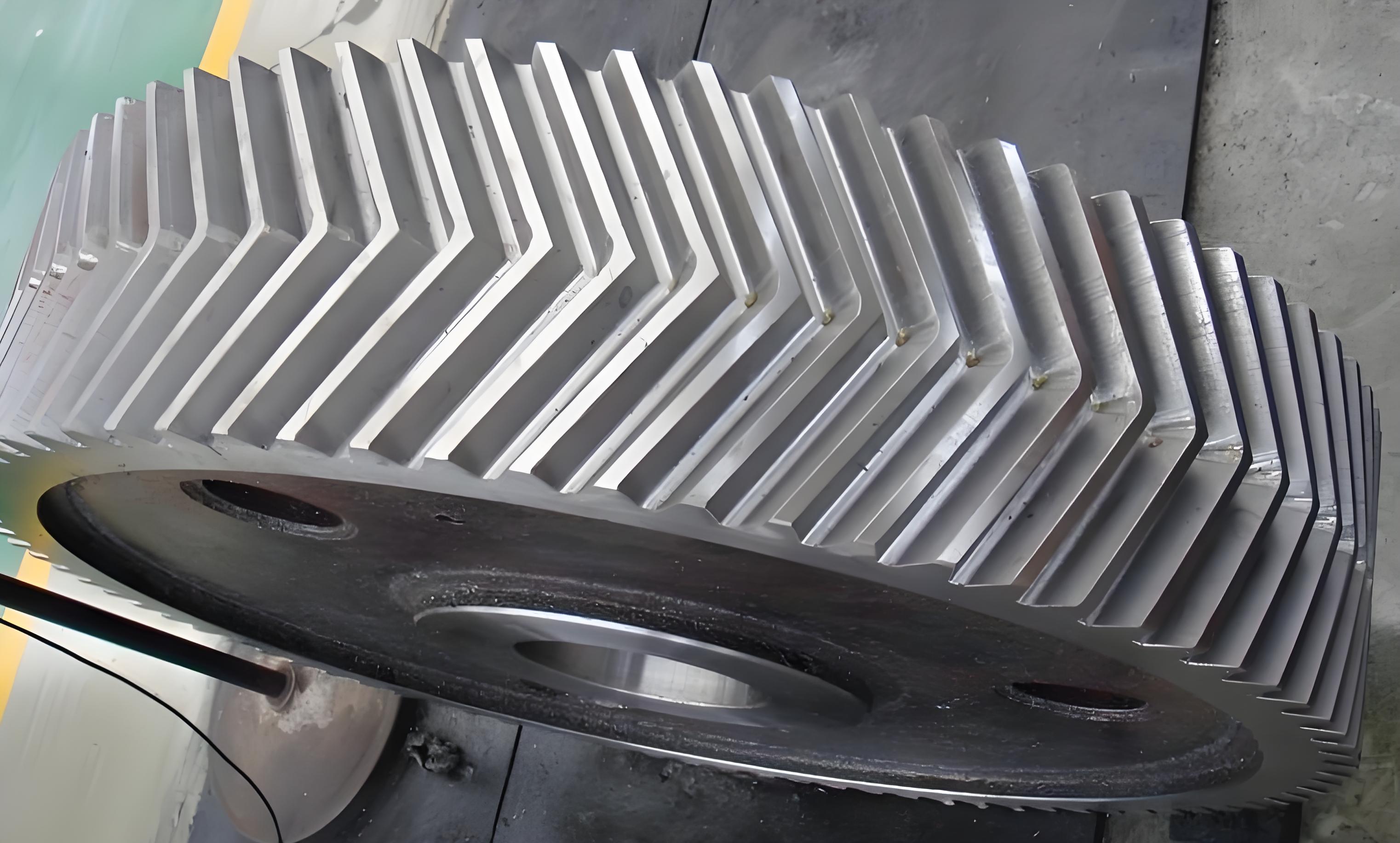
I applied this model to a specific marine herringbone gear pair, with parameters summarized in the table below. These parameters serve as the basis for my simulations and analyses, highlighting the relevance of herringbone gear systems in practical applications.
| Parameter | Driving Gear | Driven Gear |
|---|---|---|
| Normal Module (mm) | 8 | 8 |
| Normal Pressure Angle (°) | 20 | 20 |
| Helix Angle, $\beta$ (°) | 16.26 | 16.26 |
| Backlash (μm) | 2 | 2 |
| Load Torque (N·m) | 1088 | 1088 |
| Damping Ratio | 0.1 | 0.1 |
| Density (g/cm³) | 7.85 | 7.85 |
| Number of Teeth | 16 | 32 |
| Hand of Helix | Left/Right | Right/Left |
| Face Width (mm) | 35 | 35 |
| Moment of Inertia (kg·m²) | 0.049 | 2.600 |
| Operating Speed (r/min) | 1000 | 500 |
To solve the dynamic equations, I employed a variable-step fourth-order Runge-Kutta numerical integration method. This approach provided the displacement responses, which were then used to compute the dynamic load over time. For example, the dynamic load for the left helical segment during a meshing cycle is shown in subsequent analyses, with time zero corresponding to the start of meshing for the observed tooth pair. The results indicate significant fluctuations due to the nonlinear excitations, underscoring the complexity of herringbone gear dynamics.
Building on the dynamic load calculations, I developed a novel method for determining tooth root dynamic stress in herringbone gears. Traditional methods include approximate material mechanics formulas and finite element analysis, but these often lack accuracy or efficiency when dealing with dynamic loads in herringbone gear systems. My method leverages LTCA to compute the stress influence coefficient $\sigma_{ei}$ at the tooth root midpoint on the tension side of the driven gear under unit load. The dynamic stress $\sigma_{vi}$ for the $i$-th meshing contact line is then given by:
$$\sigma_{vi} = F_{vi} \cdot \sigma_{ei} \quad \text{for} \quad i = 1, \dots, n$$
where $F_{vi}$ is the dynamic load allocated to the single tooth pair at the $i$-th contact line, and $n$ is the number of contact lines considered from meshing-in to meshing-out. The key innovation lies in accurately determining $F_{vi}$ by accounting for real-time dynamic load effects on the load distribution coefficient. I explored three approaches: using static load distribution coefficients (inefficient), recalculating coefficients for each instantaneous load (accurate but slow), and a fitted relationship based on precomputed coefficients at multiple load levels. I adopted the third approach for its balance of accuracy and efficiency. Specifically, I divided the dynamic load range from minimum to maximum into five equal segments, used LTCA to obtain load distribution coefficients for each segment, and fitted a function to interpolate coefficients for any load. This allows precise calculation of $F_{vi}$ throughout the meshing cycle, capturing the true stress fluctuations in herringbone gear teeth.
For instance, for the left helical segment of the herringbone gear pair, the dynamic load on a single tooth pair during meshing was computed as a function of the driving gear’s rotation angle. The results show that the load varies significantly due to time-varying stiffness and impact forces, emphasizing the need for dynamic analysis in herringbone gear systems.
To validate my numerical simulations, I conducted experimental tests using a gear vibration testing apparatus. The setup included a motor, gearbox, test gearbox with the herringbone gear pair, and a magnetic powder brake for load application. Strain gauges were attached at the tooth root midpoint on the tension side of the driven gear to measure dynamic stress. The data acquisition system recorded stress signals, which were compared with simulation results. This experimental configuration ensures realistic conditions for evaluating herringbone gear performance under dynamic loads.
I analyzed the effects of external load torque and input speed on tooth root dynamic stress. For load torque variations, I considered three scenarios: 1500 N·m, 3000 N·m, and 4500 N·m, with a constant driving speed of 4500 r/min. The numerical and experimental results for the left helical segment’s driven gear tooth root stress are summarized below. The stress values are presented as functions of meshing angle, with key metrics extracted for comparison.
| Load Torque (N·m) | Maximum Dynamic Stress (Simulation, MPa) | Maximum Dynamic Stress (Experiment, MPa) | Error (%) | Relative Fluctuation Trend |
|---|---|---|---|---|
| 1500 | 23.64 | 25.7 | 8.0 | High due to backlash influence |
| 3000 | 54.86 | 60.0 | 8.6 | Decreased as backlash effects reduced |
| 4500 | 69.34 | 72.6 | 4.5 | Increased slightly as system entered linear region |
The data show that as load torque increases, the maximum tooth root dynamic stress rises, consistent with expectations for herringbone gear systems. However, the relative stress fluctuations initially decrease and then increase with higher loads. This non-monotonic behavior is attributed to backlash: at lower loads (e.g., 1500 N·m), tooth deformation is insufficient to eliminate backlash, causing pronounced dynamic effects and high fluctuations; at moderate loads (e.g., 3000 N·m), backlash is partially compensated, reducing fluctuations; at high loads (e.g., 4500 N·m), backlash is nearly eliminated, but other nonlinearities may dominate, leading to increased fluctuations. The simulation results align well with experimental measurements, with errors below 9%, primarily due to manufacturing tolerances, thermal deformations, and strain gauge sensitivities in herringbone gear tests.
For speed variations, I examined three cases: driving speeds of 1500 r/min, 2000 r/min, and 2500 r/min, with a constant load torque of 1088 N·m. The results are summarized in the following table, highlighting the impact of rotational speed on herringbone gear dynamic stress.
| Input Speed (r/min) | Maximum Dynamic Stress (Simulation, MPa) | Maximum Dynamic Stress (Experiment, MPa) | Error (%) | Stress Fluctuation Intensity |
|---|---|---|---|---|
| 1500 | 90.20 | 93.7 | 3.7 | Moderate |
| 2000 | 94.60 | 103.5 | 8.6 | Increased |
| 2500 | 98.68 | 107.1 | 7.9 | High |
These results demonstrate that higher input speeds lead to greater maximum dynamic stress and more pronounced stress fluctuations in herringbone gear systems. This is because increased speed amplifies inertial effects and meshing impact forces, exacerbating dynamic responses. The simulation accuracy remains acceptable, with errors under 9%, validating my model’s capability to predict herringbone gear behavior across operational ranges. Notably, discrepancies near meshing-in and meshing-out points (at angles around ±11.5°) are larger in experiments, likely due to enhanced impact forces from practical factors like gear errors and thermal effects, which are challenging to fully capture in simulations for herringbone gears.
To further illustrate the dynamic load distribution, I derived the load-sharing ratio among multiple tooth pairs in the herringbone gear system. Using the fitted approach, the instantaneous load on each contact line can be expressed as a function of the total dynamic load $F_d$ and the meshing position. For simplicity, consider a two-tooth pair meshing scenario; the load distribution coefficients $\alpha_i$ for the $i$-th pair satisfy $\sum \alpha_i = 1$. From LTCA, I obtained coefficients at five load levels and fitted a polynomial relation:
$$\alpha_i(F_d) = a_{0i} + a_{1i} F_d + a_{2i} F_d^2 + \cdots$$
where $a_{ji}$ are fitting constants. This allows real-time computation of $F_{vi} = \alpha_i(F_d) \cdot F_d$ during simulation, ensuring accurate stress calculations. The table below provides an example of fitted coefficients for the first two contact lines in the herringbone gear pair, based on normalized loads.
| Contact Line Index, $i$ | $a_{0i}$ | $a_{1i}$ (1/N) | $a_{2i}$ (1/N²) | Range of $F_d$ (N) |
|---|---|---|---|---|
| 1 | 0.55 | 2.5e-6 | -1.0e-12 | 20000 to 60000 |
| 2 | 0.45 | -2.5e-6 | 1.0e-12 | 20000 to 60000 |
These coefficients highlight how load distribution shifts with dynamic loads, a critical aspect for herringbone gear durability. For instance, at lower loads, the first contact line may carry more load, but as load increases, the distribution evens out due to deformation effects. This dynamic redistribution directly influences tooth root stress patterns, underscoring the importance of my method for herringbone gear design.
In terms of mathematical modeling, the time-varying meshing stiffness $k_m(t)$ is a key input. I computed it via LTCA by analyzing contact forces and deformations over a meshing cycle. For a herringbone gear with contact ratio $\varepsilon$, the stiffness can be approximated as a Fourier series:
$$k_m(t) = k_0 + \sum_{j=1}^{M} \left[ a_j \cos(j \omega_m t) + b_j \sin(j \omega_m t) \right]$$
where $k_0$ is the mean stiffness, $\omega_m$ is the meshing frequency, and $a_j$, $b_j$ are coefficients from LTCA. For the studied herringbone gear, $k_0 \approx 1.2 \times 10^9$ N/m, with variations up to 20% during meshing. This stiffness profile, combined with backlash nonlinearity, leads to complex dynamic responses that my model captures effectively.
To enhance the discussion, I also considered the impact of damping on herringbone gear dynamics. The equivalent damping $c_m$ in the meshing direction is estimated based on material properties and gear geometry. A common formula is $c_m = 2 \zeta \sqrt{k_m m_e}$, where $\zeta$ is the damping ratio (set to 0.1 in this study) and $m_e$ is the equivalent mass of the herringbone gear pair. For the given parameters, $m_e \approx \frac{I_p I_g}{I_p R_g^2 + I_g R_p^2}$, yielding $c_m \approx 1.5 \times 10^4$ N·s/m. Sensitivity analyses show that variations in damping can moderate stress fluctuations, but the overall trends remain consistent, affirming the robustness of my approach for herringbone gear systems.
In conclusion, my research presents a comprehensive framework for analyzing tooth root dynamic stress in herringbone gear systems. I developed a detailed 12-DOF nonlinear dynamic model that incorporates multiple excitations relevant to herringbone gears, such as time-varying stiffness, backlash, and impact forces. The proposed method for calculating dynamic stress considers real-time load distribution effects, improving accuracy while maintaining computational efficiency. Validation through experimental tests confirms that the simulations reliably predict stress trends under varying loads and speeds. Key findings include: (1) increasing external load or input speed generally raises maximum dynamic stress in herringbone gears; (2) backlash induces non-monotonic fluctuations in stress relative to load changes; and (3) the model achieves good agreement with experiments, with errors below 9%. These insights can guide the design and optimization of herringbone gear transmissions for enhanced durability and performance in demanding applications. Future work may extend the model to include thermal effects, wear, or more complex herringbone gear configurations to further advance the understanding of these critical mechanical systems.