
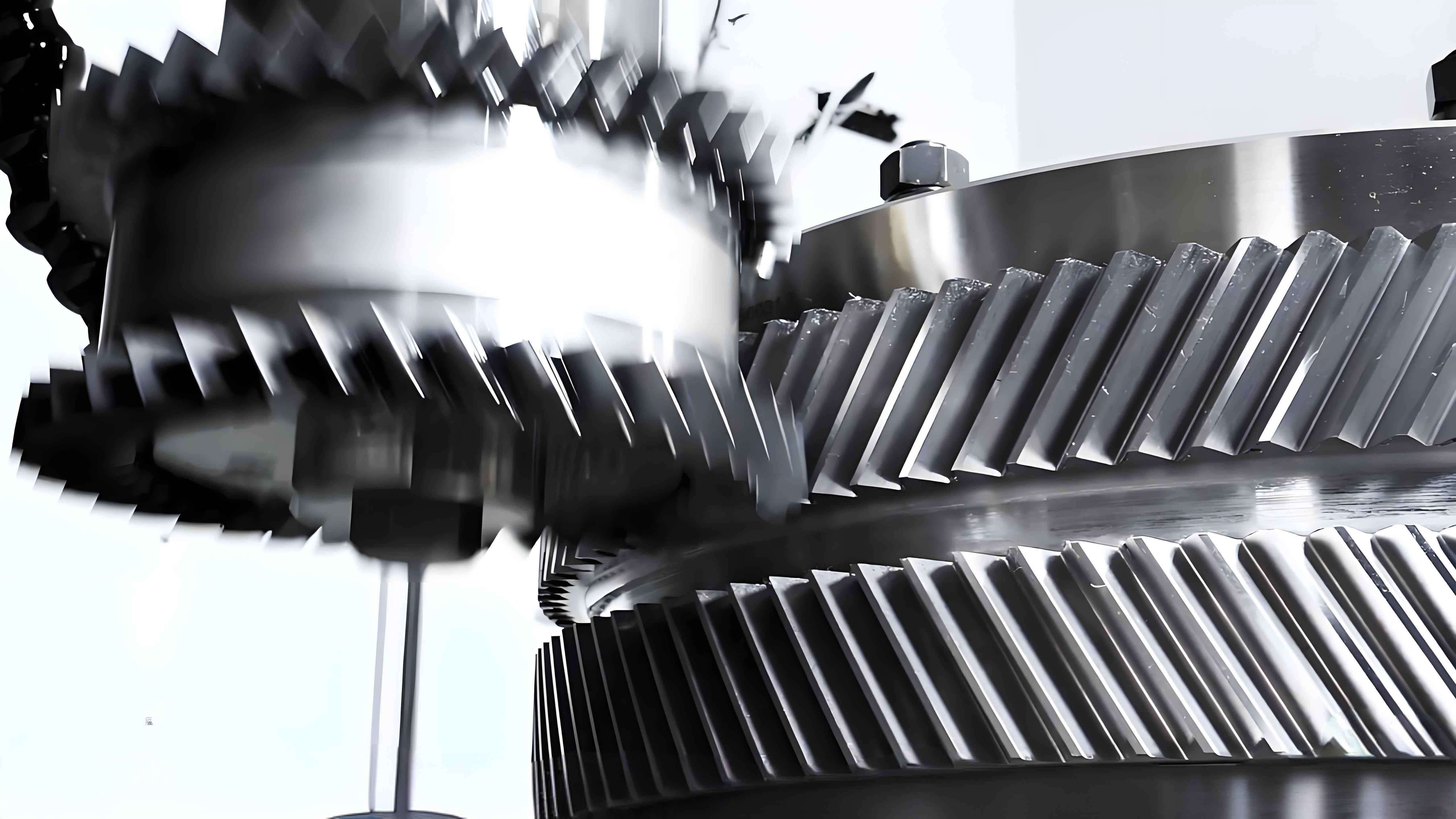
In modern high-power, high-speed transmission systems, such as those found in marine propulsion, aerospace, and heavy industrial machinery, the demands for compact design, high load capacity, and operational smoothness are paramount. Traditional single-path transmissions often reach their limits in such demanding applications. To overcome these limitations, power branching configurations have been developed. These systems distribute the input power across multiple parallel paths before recombining it at the output, effectively reducing the load on individual gear meshes and allowing for more compact and lightweight designs. Among the various gear types suitable for such tasks, the herringbone gear stands out due to its inherent ability to cancel out axial thrust forces, leading to smoother operation and reduced bearing loads, which is critical for high-speed applications.
While dual-branch systems have been studied extensively, the progression to a triple-branch configuration represents a significant step forward in enhancing power density and reliability. This research focuses on the modeling and simulation of a specific triple-branch transmission system incorporating herringbone gears. The system’s core innovation lies in integrating a planetary gear stage as the third branch alongside two conventional parallel paths. The primary challenge in such multi-branch systems is achieving equal load sharing among all branches. Manufacturing inaccuracies, assembly errors, and minute deflections under load can disrupt this balance, leading to one path carrying a disproportionate share of the power, which ultimately reduces the system’s overall life and reliability.
This article presents a comprehensive simulation methodology to analyze the power flow distribution within a herringbone gear triple-branch transmission under various operational and error conditions. By developing a detailed mathematical model that accounts for the complex interactions between gear mesh stiffness, shaft compliances, and system kinematics, we can predict how power is divided at any given moment during the gear meshing cycle. The goal is to provide a robust analytical tool that can inform the design and error budgeting for such advanced transmission systems, ensuring optimal performance and durability.
System Configuration and Mathematical Modeling
Transmission Principle
The triple-branch transmission system under investigation is designed to split input power three ways. The schematic layout is based on an evolution from a dual-branch design, where a planetary gear train is ingeniously inserted as the third power path. Input power is delivered to a primary pinion (Gear 1). This pinion simultaneously drives two primary large gears (Gears 2 and 3) in a conventional parallel arrangement. These two paths constitute Branch I and Branch II. The third branch (Branch III) is created by connecting the input shaft, via a flexible coupling and a through-shaft, to the sun gear of a planetary stage. The planetary carrier is fixed. The rotation of the sun gear drives the planet gears, which in turn drive the ring gear. The output from the ring gear is then coupled to a secondary pinion.
All three secondary pinions (two from the parallel branches and one from the planetary branch) then mesh with a single, common secondary large gear (Gear 7), recombining the power into a single output. This configuration allows a single input herringbone gear to drive three separate secondary pinions, significantly increasing the system’s potential torque capacity while maintaining a relatively compact envelope.
Mathematical Formulation of System Mechanics
To analyze this complex system, a lumped-parameter model is developed. The system’s state is analyzed at discrete positions within the meshing cycle of the herringbone gears, as the load-sharing characteristics vary with the changing contact conditions along the tooth flank. For a given meshing position \( k \) (where \( k = 1, 2, …, N \), and \( N \) is the number of discrete positions per cycle, typically 5), we establish the governing equations.
1. Torque Equilibrium Equations:
Based on the static force balance of the system components, the following equations hold for the input torque \( T_{in} \) and the torques transmitted by each gear pair \( T_{ij} \) (torque on gear \( i \) from gear \( j \)):
$$ T_{in} + T_{12}^k + T_{13}^k + T_{18}^k = 0 $$
$$ T_{47}^k – T_{12}^k \cdot (Z_2 / Z_1) = 0 $$
$$ T_{57}^k – T_{13}^k \cdot (Z_3 / Z_1) = 0 $$
$$ T_{67}^k – T_{18}^k \cdot (Z_8 / Z_1) = 0 $$
Here, \( Z_i \) denotes the number of teeth for gear \( i \). Gears 8, 10, 11 are the sun, planet, and ring of the planetary stage, with an equivalent ratio reflected in \( Z_8 / Z_1 \).
2. Deformation Compatibility Equations:
The angular deflections experienced by each power path from the input to the final output mesh must be compatible, as they all drive the same output gear (Gear 7). This compatibility condition is crucial for determining how the load is shared. For any two branches, their total angular deflection from the input split point to the point of force application on Gear 7 must be equal. This leads to the following equations for the \( k \)-th mesh position:
$$ \delta_{12}(T_{12}^k) \cdot \frac{Z_1}{Z_2} + \delta_{24}(T_{12}^k) \cdot \frac{Z_2}{Z_1} + \delta_{47}(T_{47}^k) = \delta_{13}(T_{13}^k) \cdot \frac{Z_1}{Z_3} + \delta_{35}(T_{13}^k) \cdot \frac{Z_3}{Z_1} + \delta_{57}(T_{57}^k) $$
$$ \delta_{12}(T_{12}^k) \cdot \frac{Z_1}{Z_2} + \delta_{24}(T_{12}^k) \cdot \frac{Z_2}{Z_1} + \delta_{47}(T_{47}^k) = \delta_{18}(T_{18}^k) \cdot \frac{Z_1}{Z_2} + \delta_{86}(T_{18}^k) \cdot \frac{Z_8}{Z_1} + \delta_{67}(T_{67}^k) $$
In these equations, \( \delta_{ij}(T) \) represents the total angular deformation of the component(s) between nodes \( i \) and \( j \) as a function of the transmitted torque \( T \). This includes both the torsional wind-up of shafts (like 2-4, 3-5, 8-6) and, most importantly, the loaded composite deformation of the herringbone gear mesh itself (like 1-2, 4-7).
Simulation Methodology for Power Flow Analysis
Modeling Gear Mesh and Shaft Compliance
The core of the simulation lies in accurately defining the function \( \delta_{ij}(T) \), particularly for the gear meshes. For a herringbone gear pair, the loaded transmission error (LTE) under torque is a non-linear function comprising three main components:
- Geometric Transmission Error (\( \Delta_1 \)): A constant determined by the design and manufacturing of the tooth surfaces, independent of load.
- Bending/Shear Deformation (\( \Delta_2 \)): Assumed to be linearly proportional to the applied load \( T \).
- Contact Deformation (\( \Delta_3 \)): Based on Hertzian contact theory, proportional to \( T^{2/3} \).
Therefore, the angular deformation for a gear mesh can be modeled as:
$$ \delta_{mesh}(T) = A + B \cdot T + C \cdot T^{2/3} $$
where \( A \) encapsulates \( \Delta_1 \), \( B \) is the linear compliance coefficient, and \( C \) is the contact compliance coefficient.
For torsional shafts, the deformation is typically linear:
$$ \delta_{shaft}(T) = D \cdot T $$
where \( D \) is the torsional compliance of the shaft.
The coefficients \( A, B, C, D \) are unique for each component and vary with the meshing position \( k \) for gear pairs due to changing contact geometry. They are determined offline through a combination of Finite Element Analysis (FEA) and Loaded Tooth Contact Analysis (LTCA) for the herringbone gear pairs. The LTCA is performed at the discrete meshing positions for three representative load levels (e.g., 0.1\(T_{in}\), 0.5\(T_{in}\), 0.9\(T_{in}\)) to fit the non-linear function and obtain \( A^k, B^k, C^k \) for each mesh \( k \).
Power Flow Solution via Optimization
With the compliance functions established, the system of equations (Torque Equilibrium and Deformation Compatibility) must be solved for the unknown torques \( T_{12}^k, T_{13}^k, T_{18}^k, T_{47}^k, T_{57}^k, T_{67}^k \) at each meshing position \( k \). This constitutes a non-linear system where direct solution is complex. An effective approach is to transform it into an optimization problem.
For each meshing position \( k \), we define an optimization model. The design variables are the gear mesh torques. The objective is to minimize the violation of the deformation compatibility equations, effectively seeking the torque distribution that makes the total deflection of all paths equal. The torque equilibrium equations and the sign conventions from the compliance functions serve as constraints.
The optimization problem for position \( k \) can be formally stated as:
$$ \min \left[ \left( \delta_{12}^k + \delta_{24}^k + \delta_{47}^k – \delta_{13}^k – \delta_{35}^k – \delta_{57}^k \right)^2 + \left( \delta_{12}^k + \delta_{24}^k + \delta_{47}^k – \delta_{18}^k – \delta_{86}^k – \delta_{67}^k \right)^2 \right] $$
Subject to:
$$ T_{in} + T_{12}^k + T_{13}^k + T_{18}^k = 0 $$
$$ T_{47}^k = T_{12}^k \cdot (Z_2 / Z_1) $$
$$ T_{57}^k = T_{13}^k \cdot (Z_3 / Z_1) $$
$$ T_{67}^k = T_{18}^k \cdot (Z_8 / Z_1) $$
$$ \delta_{ij}^k = f_{ij}^k(T_{ij}^k) $$
Solving this optimization problem for all \( k \) meshing positions using a numerical method like the Newton-Raphson algorithm yields the instantaneous power flow (torque distribution) throughout the entire meshing cycle. The power in each branch is simply \( P_{ij}^k = T_{ij}^k \cdot \omega \).
Simulation Case Study and Results Analysis
A simulation was conducted for a system with an input power of 1556 kW at 6000 RPM. The key geometric and material parameters for the herringbone gears in the system are summarized below:
| Parameter | Pinion 1 | Gears 2, 3, 8 | Pinions 4,5,6 | Gear 7 |
|---|---|---|---|---|
| Number of Teeth | 28 | 66 | 32 | 84 |
| Normal Module (mm) | 6 | 6 | 6 | 6 |
| Pressure Angle (°) | 20 | 20 | 20 | 20 |
| Helix Angle (°) | 29.5 | 29.5 | 29.5 | 29.5 |
| Face Width (mm) | 120 | 110 | 120 | 110 |
| Young’s Modulus (GPa) | 210 | 210 | 210 | 210 |
| Poisson’s Ratio | 0.3 | 0.3 | 0.3 | 0.3 |
The simulation was run for several scenarios: a nominal “perfect” assembly, and various cases with simulated assembly errors (e.g., misalignment) introduced into specific gear meshes. The power flow through the primary branches (\(T_{12}, T_{13}, T_{18}\)) and the corresponding secondary meshes (\(T_{47}, T_{57}, T_{67}\)) was calculated over two complete meshing cycles.
Key Findings:
- Nominal (Error-Free) Condition: As expected, the power is almost perfectly equally divided among the three branches at every meshing position. The slight oscillations visible in the power flow graphs are due to the periodic variation in mesh stiffness of the herringbone gear pairs as different tooth regions come into contact.
- Effect of Isolated Assembly Errors: When an assembly error is introduced in a specific mesh (e.g., the mesh between Gears 1 and 2), the load sharing is disrupted. The branch containing the erroneous mesh and its associated downstream path sees a significant shift in its load-carrying proportion, which now fluctuates above and below the nominal value. The other branches adjust accordingly to maintain equilibrium.
- Cumulative Effect of Errors: The most significant imbalance occurs when all gear meshes are assumed to have assembly errors simultaneously. The combined effect leads to pronounced and complex fluctuations in the power flow of each branch. The load is no longer evenly shared, and one branch may be consistently overloaded while another is underloaded, posing a serious risk to system longevity.
- Sensitivity: The simulation clearly shows that errors in the secondary stage meshes (e.g., 4-7, 5-7, 6-7) have a more pronounced effect on power split imbalance than equivalent errors in the primary stage for this particular configuration. This highlights critical areas for manufacturing and assembly control.
| Condition | Primary Branch Power Flow | Secondary Mesh Power Flow | Overall Imbalance Severity |
|---|---|---|---|
| Nominal (Perfect) | Near-perfect equal split, minor cyclic variation. | Near-perfect equal split, follows primary branch. | Very Low |
| Error in Mesh 1-2 | Branch I (T12) deviates. Branches II & III adjust. | Mesh 4-7 deviates accordingly. | Moderate |
| Error in Mesh 4-7 | Branch I (T12) deviates. Similar to above but more pronounced. | Mesh 4-7 shows significant deviation. | High |
| Combined Errors (All Meshes) | All three branches show significant, unique fluctuating patterns. | All secondary meshes show correlated significant fluctuations. | Very High |
Discussion and Conclusion
The simulation study demonstrates the efficacy of the proposed methodology for analyzing complex power branching systems employing herringbone gears. The developed model successfully captures the dynamic load-sharing behavior that varies within a single mesh cycle due to changing tooth compliance. The results underscore several critical engineering insights.
Firstly, the triple-branch configuration intrinsically offers a high load capacity by dividing the input torque three ways instead of two or one. However, its performance is highly sensitive to manufacturing and assembly precision. The goal of “equal load sharing” is difficult to achieve in practice without careful design of flexible couplings, tolerance management, and potentially phased gear assembly. The presented simulation tool allows designers to quantify the impact of various error budgets on system performance before physical prototyping.
Secondly, the non-linear compliance of the herringbone gear mesh, particularly the Hertzian contact deformation term (\(T^{2/3}\)), is essential for accurate prediction. A purely linear stiffness model would fail to predict the correct load distribution, especially under high loads.
In conclusion, this research provides a robust simulation framework for the power flow analysis of advanced herringbone gear triple-branch transmission systems. By solving the non-linear optimization model derived from force equilibrium and deformation compatibility, we can predict the intricate power split under both ideal and realistic error conditions. The findings highlight that while the triple-branch structure significantly enhances potential power density, its successful implementation hinges on managing system compliance and minimizing assembly errors to ensure acceptable load distribution. This work lays a foundation for the design optimization and reliability assessment of such high-performance transmission systems, confirming their significant engineering application value in fields demanding compact, high-torque, and high-speed power transmission solutions.