
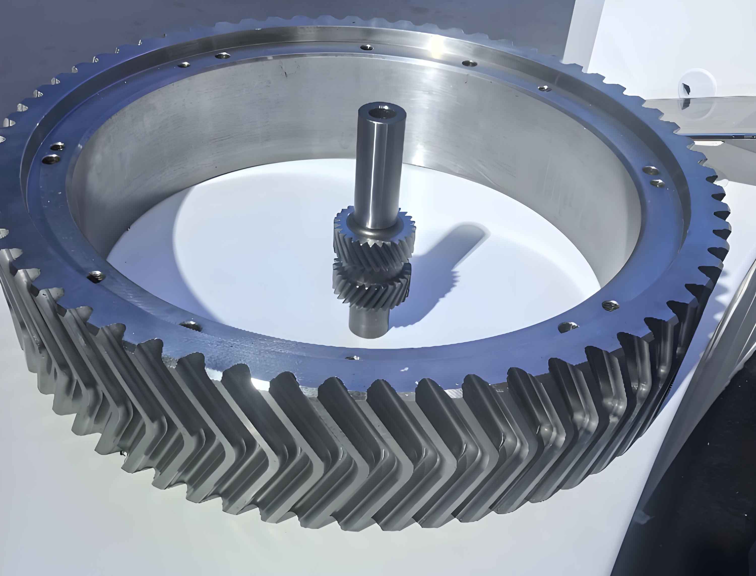
In the design of high-performance power transmission systems, particularly those demanding exceptional smoothness and low noise such as marine propulsion units, herringbone gears with high contact ratios are often the component of choice. A critical internal parameter governing the dynamic behavior of any gear system is the mesh stiffness. For conventional gears with low to moderate contact ratios, established analytical formulas provide satisfactory estimates. However, for herringbone gears where the contact ratio can reach 5 or higher, these formulas break down due to the complex, multi-tooth engagement state and the significant influence of the gear body structure. In such cases, numerical methods like the Finite Element Method (FEM) become necessary. While accurate, this approach creates a significant bottleneck: the computational process is lengthy, the model size explodes, and it becomes profoundly difficult to discern the underlying, often non-linear, influence rules of multiple design and structural parameters on the resulting mesh stiffness from the scattered simulation data.
This is where the paradigm of Knowledge Discovery in Databases (KDD), or more specifically, in simulation data, becomes invaluable. While CAE tools are excellent for design verification, they typically do not automatically extract the latent, actionable knowledge embedded within the simulation results. The goal shifts from merely computing a value for a given set of inputs to discovering the generalized relationships between inputs and outputs. This work presents a methodology that synergistically combines Fuzzy Clustering and Rough Set Theory (RST) to mine design knowledge from the simulation data of high-contact-ratio herringbone gears, explicitly deriving decision rules that link key parameters to categorized levels of mesh stiffness.
Methodological Foundation: Fuzzy Clustering and Rough Set Theory
Fuzzy C-Means Clustering
To begin the knowledge discovery process, we first need to categorize the continuous output variable—the gear pair’s mesh stiffness. Fuzzy logic, introduced by Zadeh, provides a natural framework for handling the inherent ambiguity in classifying a continuous value. Instead of a hard, binary assignment, fuzzy clustering allows a data point to belong to multiple clusters with varying degrees of membership.
Let the set of simulation objects (data points) be \( P = \{ p_1, p_2, …, p_n \} \), where each \( p_k \) represents a unique combination of design parameters and its corresponding calculated mesh stiffness. The objective is to partition this set into \( c \) clusters. The Fuzzy C-Means (FCM) algorithm, an extension of the ISODATA technique, aims to find the optimal fuzzy partition matrix \( R = [r_{ik}] \) and the cluster center matrix \( M = [M_1, M_2, …, M_c]^T \) by minimizing the following objective function:
$$J(R, M) = \sum_{k=1}^{n} \sum_{i=1}^{c} r_{ik}^q \| \mathbf{p}_k – \mathbf{M}_i \|^2$$
where:
- \( r_{ik} \in [0,1] \) is the membership degree of object \( p_k \) to cluster \( i \),
- \( q > 1 \) is the fuzzifier (typically set to 2),
- \( \| \mathbf{p}_k – \mathbf{M}_i \| \) is the Euclidean distance between object \( p_k \) and cluster center \( \mathbf{M}_i \).
- The constraints are \( \sum_{i=1}^{c} r_{ik} = 1 \) for all \( k \) and \( \sum_{k=1}^{n} r_{ik} > 0 \) for all \( i \).
The quality of the fuzzy partition is evaluated using the Classification Coefficient \( F(R) \) and the Average Fuzzy Entropy \( H(R) \):
$$F(R) = \frac{1}{n} \sum_{k=1}^{n} \sum_{i=1}^{c} r_{ik}^2$$
$$H(R) = -\frac{1}{n} \sum_{k=1}^{n} \sum_{i=1}^{c} r_{ik} \ln(r_{ik})$$
A value of \( F(R) \) close to 1 and \( H(R) \) close to 0 indicates a well-defined, effective clustering result.
Rough Set Theory for Rule Induction
Once the mesh stiffness is categorized, the problem transforms into learning decision rules from a table of examples. Rough Set Theory (RST), pioneered by Pawlak, is a powerful mathematical tool for this purpose. It handles uncertainty and vagueness without needing external, a priori information (like probability distributions), making it ideal for mining deterministic rules from crisp or discretized data.
The core structure in RST is a decision table \( S = (U, Z, V, f) \), where:
- \( U = \{ x_1, x_2, …, x_n \} \) is the universe (the set of simulation cases).
- \( Z = T \cup D \) is a finite set of attributes, with \( T \) being the set of condition attributes (design parameters) and \( D \) being the set of decision attributes (mesh stiffness class), such that \( T \cap D = \emptyset \).
- \( V = \bigcup_{r \in Z} V_r \) is the set of all attribute values.
- \( f: U \times Z \rightarrow V \) is an information function assigning a value to each attribute for every object.
The goal is to reduce the decision table to its most informative core and extract concise decision rules. This involves two key steps:
- Attribute Reduction: Finding a minimal subset of condition attributes \( Red \subseteq T \) that preserves the same classificatory power as the full set \( T \) with respect to \( D \). The indispensable attributes form the core \( Core_T(D) \). The importance of an attribute \( r \in T \) is measured by the change in classification quality if it is removed:
$$\sigma_{(T, D)}(r) = \frac{\gamma_T(D) – \gamma_{T-\{r\}}(D)}{\gamma_T(D)}$$
where \( \gamma \) represents the quality of classification (the proportion of objects correctly classified based on the indiscernibility relation). - Attribute Value Reduction: Further simplifying each rule in the reduced table by removing superfluous attribute values. The result is a set of minimal decision rules of the form \( \text{(Condition)} \rightarrow \text{(Decision)} \).
The certainty of a rule \( A \rightarrow B \) is quantified by its confidence factor \( CF \):
$$CF(A \rightarrow B) = \frac{|[x]_A \cap [x]_B|}{|[x]_A|}$$
where \( [x]_A \) is the set of objects matching condition \( A \), and \( [x]_B \) is the set of objects matching decision \( B \).
Analysis of Design Parameters for Herringbone Gear Mesh Stiffness
The herringbone gear pair’s mesh stiffness is not solely a function of tooth geometry. For high-contact-ratio gears operating under significant loads, the compliance of the gear body (web, rim, etc.) substantially influences the overall mesh stiffness. Therefore, our analysis must integrate both macro-geometry design parameters and meso-scale structural parameters of the gear blank.
Through a detailed parametric modeling and FEM-based simulation workflow, 51 distinct design cases were generated. The following 13 parameters were selected as condition attributes (T), with the average mesh stiffness over an engagement cycle as the decision attribute (D).
| Type | Parameter Name | Symbol |
|---|---|---|
| Condition Attributes (T) | Rim Thickness | \( S_R \) |
| Web Thickness | \( b_s \) | |
| Number of Lightening Holes | \( n \) | |
| Radius of Lightening Holes | \( D_W \) | |
| Module | \( m \) | |
| Addendum Coefficient | \( h_a^* \) | |
| Helix Angle | \( \beta \) | |
| Face Width | \( B \) | |
| Pinion Tooth Number | \( z_1 \) | |
| Gear Tooth Number | \( z_2 \) | |
| Transverse Contact Ratio | \( \epsilon_{\alpha} \) | |
| Total Contact Ratio | \( \epsilon \) | |
| Mesh Type (External=1, Internal=0) | \( T \) | |
| Decision Attribute (D) | Gear Pair Mesh Stiffness | \( C \) |
Fuzzy Clustering of Mesh Stiffness
Applying the FCM algorithm to the 51 calculated mesh stiffness values with a predefined cluster number \( c = 7 \), we obtain the following cluster centers after iteration:
$$ M = [18.8872, \; 20.3133, \; 21.6716, \; 22.6145, \; 24.2252, \; 25.8344, \; 28.4950]^T $$
These centers, labeled C1 through C7, represent the characteristic stiffness levels. The clustering results are:
- C1: 5 cases
- C2: 12 cases
- C3: 10 cases
- C4: 4 cases
- C5: 5 cases
- C6: 11 cases
- C7: 4 cases
The clustering quality metrics are \( F(R) = 0.9968 \) and \( H(R) = 0.0066 \), confirming an excellent and well-defined partition. This categorization transforms the continuous stiffness value into a discrete decision class \( D \), which is essential for the subsequent RST analysis.
Knowledge Discovery Process and Rule Derivation
The core of the knowledge discovery from the herringbone gear simulation data involves processing the decision table through the RST pipeline.
1. Decision Table Discretization
RST requires discrete-valued attributes. All 13 continuous condition attributes (\( S_R, b_s, …, \epsilon \)) were discretized into 3 to 5 intervals using a suitable algorithm (e.g., Boolean reasoning combined with RST) that finds cut-points without introducing conflicts into the decision table. The decision attribute \( D \) is already discrete with 7 classes from the fuzzy clustering.
2. Attribute Reduction
Performing attribute reduction on the discretized table reveals which parameters are truly indispensable for determining the mesh stiffness class.
Core Attributes \( Core_T(D) \): These are the absolutely essential parameters. The analysis identified:
$$ Core_T(D) = \{ S_R, \; b_s, \; n, \; D_W, \; h_a^* \} $$
This implies that Rim Thickness, Web Thickness, Number of Lightening Holes, their Radius, and the Addendum Coefficient form the fundamental set of factors that cannot be removed without losing essential classificatory information about the mesh stiffness of these herringbone gears.
One Relative Reduct \( Red_T(D) \): A larger, minimal set that retains full classificatory power but is more convenient for rule generation was found:
$$ Red_T(D) = \{ S_R, \; b_s, \; n, \; D_W, \; m, \; h_a^*, \; z_1, \; \epsilon, \; T \} $$
This reduct includes the core plus Module, Pinion Tooth Number, Total Contact Ratio, and Mesh Type. Notably, parameters like Helix Angle (\( \beta \)) and Face Width (\( B \)) were deemed redundant in the presence of others within this specific dataset, significantly simplifying the rule discovery space.
3. Attribute Value Reduction and Rule Generation
Using the relative reduct \( Red_T(D) \), attribute value reduction is performed to eliminate superfluous conditions from each row of the decision table. This yields a set of minimal decision rules. From the initial 51 cases, 31 minimal rules were extracted. By setting a confidence threshold (e.g., 55%), a more robust and concise set of 14 key decision rules is obtained. Their confidence factors are calculated as per Equation (4).
| Rule # | Condition (IF) | Decision (THEN Stiffness Class) | Confidence |
|---|---|---|---|
| 1 | Rim Thickness is Level 1 AND Pinion Teeth is Level 2 | C2 | 100% |
| 2 | Rim Thickness is Level 4 AND Pinion Teeth is Level 2 | C3 | 100% |
| 3 | Rim Thickness is Level 5 AND Pinion Teeth is Level 2 | C4 | 100% |
| 4 | Web=2, Holes=3, Hole Rad.=2, Module=2, Add. Coef.=4, Pinion Teeth=1, Total Contact Ratio=2 | C2 | 58.6% |
| 5 | Number of Lightening Holes is Level 2 AND Pinion Teeth is Level 1 | C2 | 100% |
| 6 | Web Thickness is Level 2 AND Pinion Teeth is Level 2 | C2 | 100% |
| 7 | Web Thickness is Level 1 AND Pinion Teeth is Level 1 | C1 | 100% |
| 8 | Web Thickness is Level 3 AND Pinion Teeth is Level 2 | C3 | 100% |
| 9 | Web Thickness is Level 3 AND Pinion Teeth is Level 1 | C2 | 100% |
| 10 | Web Thickness is Level 4 AND Pinion Teeth is Level 2 | C4 | 100% |
| 11 | Web Thickness is Level 5 AND Pinion Teeth is Level 2 | C5 | 100% |
| 12 | Web Thickness is Level 5 AND Pinion Teeth is Level 1 | C4 | 100% |
| 13 | Rim=3, Web=2, Holes=3, Hole Rad.=2, Module=2, Add. Coef.=4, Pinion Teeth=2, Total Cont. Ratio=4 | C4 | 66.7% |
| 14 | Addendum Coefficient is Level 2 AND Total Contact Ratio is Level 1 | C1 | 100% |
These rules provide explicit, human-readable design knowledge. For instance, Rule 11 states with full confidence that if the Web Thickness is in its highest level (Level 5) and the Pinion has a high number of teeth (Level 2), the mesh stiffness will be in the high class C5. Rules 4 and 13 have lower confidence, indicating more specific or less frequent conditions in the dataset.
Validation and Discussion
To validate the practicality of the discovered knowledge, new herringbone gear design samples outside the original 51 cases were analyzed through the full FEM workflow. Their parameters and resulting mesh stiffness are shown below.
| Sample | Key Discrete Parameters* | Calculated Avg. Stiffness | Predicted Class by Rules | Actual Cluster |
|---|---|---|---|---|
| U1 | \( S_R\)=Very Low, \( b_s\)=Med, \( n\)=High, \( z_1\)=Low | 15.27 | Not Covered | Below C1 |
| U2 | \( n\)=Level 2, \( z_1\)=Level 1 | 20.21 | C2 (by Rule 5) | C2 (20.31) |
| U3 | \( b_s\)=Level 4, \( z_1\)=Level 2 | 22.43 | C4 (by Rule 10) | C4 (22.61) |
*After discretization according to the established cut-points.
The results are insightful:
- Sample U2: Perfectly matches the condition of Rule 5 (“Number of Lightening Holes is Level 2 AND Pinion Teeth is Level 1 → C2”). Its calculated stiffness of 20.21 falls squarely within the domain of cluster C2 (center at 20.31).
- Sample U3: Perfectly matches the condition of Rule 10 (“Web Thickness is Level 4 AND Pinion Teeth is Level 2 → C4”). Its calculated stiffness of 22.43 is very close to the C4 cluster center of 22.61.
- Sample U1: Could not be matched by any rule. This is because its Rim Thickness value fell into a discretization level not represented in the original training data (it was “Very Low” compared to the existing levels). Furthermore, its stiffness (15.27) is significantly lower than the smallest cluster center C1 (18.89), placing it outside the recognized design space.
This validation underscores both the power and the limitations of the data-driven knowledge discovery approach. The rules are highly effective for interpolation within the bounds of the knowledge space defined by the original simulation dataset. However, they cannot extrapolate to radically new design regions not sampled initially. This highlights a critical point: the quality and coverage of the discovered knowledge are directly dependent on the planning of the initial design of experiments (DoE). To build a more robust and generalizable rule base for herringbone gear design, future work must incorporate advanced DoE techniques to ensure the simulation samples are evenly distributed across the entire multi-dimensional design space of interest.
Conclusion
Determining the mesh stiffness of high-contact-ratio herringbone gears is a complex, computationally intensive task that obscures the underlying influence of multiple design parameters. This work demonstrates a effective pathway to transform numerical simulation data into explicit, actionable design knowledge. By first applying Fuzzy C-Means clustering to categorize the continuous mesh stiffness output into distinct performance classes, and then employing Rough Set Theory to mine concise decision rules from the discretized parameter space, we move from opaque computation to transparent insight.
The process successfully identified the core structural parameters (Rim Thickness, Web Thickness, lightening hole details) as fundamentally indispensable for stiffness classification. It further produced a set of simplified “IF-THEN” rules that directly link specific combinations of parameter levels to expected stiffness categories. The validation on new samples confirmed that these rules provide accurate guidance for designs falling within the explored parameter ranges.
This methodology bridges the gap between high-fidelity CAE analysis and knowledge-based engineering (KBE). For designers of herringbone gear transmission systems, such a rule set offers a rapid preliminary assessment tool, reducing dependency on full simulation cycles for every design iteration and providing intuitive guidance for achieving desired dynamic performance characteristics. Future advancements hinge on enriching the foundational simulation dataset through strategic design of experiments, thereby expanding the domain of applicability and robustness of the discovered design knowledge.