
In the realm of power transmission, gear pairs are fundamental components, and their performance is critically dependent on the nature of contact between the mating tooth surfaces. Tooth Contact Analysis (TCA) is an indispensable tool for predicting and evaluating this contact behavior, encompassing key characteristics such as the path of contact, transmission errors, and the size and shape of the contact pattern on the tooth flank. While established mathematical models for TCA exist and are widely used in industry, they encounter significant challenges under certain conditions, particularly boundary contact scenarios. This article addresses these limitations by proposing a new, robust methodology for TCA.
The primary objective of our work is to develop a comprehensive analytical framework that remains stable and accurate even when gear teeth experience boundary contact—a condition where the normal vectors at the contacting points on the two flanks do not perfectly align, often causing conventional nonlinear equation solvers to diverge. Furthermore, traditional methods that approximate the contact area using an ellipse based on local surface curvature can exhibit increasing errors as the relative misalignment between the gears grows. Our proposed method aims to circumvent these issues, providing a more general and reliable solution applicable to various gear types, especially miter gears, under arbitrary assembly and loading conditions.
Our development proceeds in two main stages. First, we establish a precise mathematical model for the tooth flanks of straight bevel gears, specifically those with a spherical involute profile. We then introduce and elaborate on our novel TCA procedure. For the gear blank design, we adhere to the formulas provided by the AGMA standard. The spherical involute profile theoretically provides line contact. However, to accommodate manufacturing inaccuracies and improve tolerance to assembly errors, tooth surface modifications (or corrections) are often applied. Deriving an explicit closed-form equation for a modified spherical involute surface is complex. Therefore, we employ a B-spline surface fitting technique to accurately represent the modified tooth flank using discrete coordinate data points, creating a new, analyzable surface equation.
To validate the correctness and effectiveness of our proposed TCA method, we will use the well-established Litvin’s method as a benchmark for comparison. By analyzing a specific case study of a pair of miter gears, we will demonstrate that our method yields consistent results for contact path and transmission error, while offering a potentially more accurate representation of the contact pattern, particularly near the edges of the tooth.
Mathematical Model of Modified Straight Bevel Gear Tooth Flanks
Spherical Involute Tooth Surface Model
The spherical involute is widely recognized as the theoretical tooth form for straight bevel gears. It can be visualized as the trace of a point on a taut string being unwound from a base circle that lies on the surface of a sphere. The mathematical model for a spherical involute tooth flank can be expressed in a parametric form. Let $r$ be the radial distance (sphere radius) and $\phi$ be the spherical involute parameter. The position vector $\mathbf{r}_s$ of a point on the spherical involute surface in its own coordinate system is given by:
$$\mathbf{r}_s(r, \phi) = \begin{bmatrix} r \sin \delta(\phi) \cos \psi(\phi) \\ r \sin \delta(\phi) \sin \psi(\phi) \\ r \cos \delta(\phi) \end{bmatrix}$$
where $\delta(\phi)$ and $\psi(\phi)$ are angular parameters defined by the geometry of the base cone and the involute development. For a standard spherical involute, these are functions of the base cone angle $\delta_b$ and the parameter $\phi$:
$$\delta(\phi) = \cos^{-1}(\cos \delta_b \cdot \cos(\sin \delta_b \cdot \phi))$$
$$\psi(\phi) = \tan^{-1}\left(\frac{\sin(\sin \delta_b \cdot \phi)}{\tan \delta_b}\right) – \phi$$
Fillet Surface Model
A complete tooth model requires a fillet surface connecting the active tooth flank to the root cone. The fillet is typically a circular arc on the sphere, tangent to both the root circle and the spherical involute profile. Its equation on the sphere can be initially defined as:
$$\mathbf{r}_c(r, \theta) = \begin{bmatrix} \rho_b \cos \theta \\ \rho_b \sin \theta \\ \sqrt{r^2 – \rho_b^2} \end{bmatrix}$$
where $\rho_b$ is the radius of the fillet circle and $\theta$ is the parameter along the circle. This circle must then be rotated and positioned correctly. A coordinate transformation matrix $\mathbf{M}_{fc}(\theta_D, \alpha_f, \delta_f)$ is applied, which involves successive rotations by angles $\theta_D$, $\alpha_f$, and $\delta_f$ to achieve tangency with the root cone and the involute flank. The final fillet surface equation is:
$$\mathbf{r}_f(\theta_D, \alpha_f, \delta_f; r, \theta) = \mathbf{M}_{fc}(\theta_D, \alpha_f, \delta_f) \cdot \mathbf{r}_c(r, \theta)$$
The parameters $(\theta_D, \alpha_f, \delta_f)$ are determined from geometric conditions of tangency, ensuring a smooth transition in the tooth model.
Tooth Surface Modification
To enhance performance and compensate for errors, the theoretical tooth surface is often modified. We apply a simple yet effective bi-directional polynomial modification. The modification amount $\delta(x, y)$ at a point located at distances $x$ (along the face width) and $y$ (along the profile height) from a reference point (often the pitch point) is defined as:
$$\delta(x, y) = a_1 + a_2 x + a_3 y + a_4 x y + a_5 x^2 + a_6 y^2$$
For our analysis, we focus on profile and longitudinal crowning. Therefore, we set the coefficients for constant, linear, and twist terms to zero: $a_1 = a_2 = a_3 = a_4 = 0$. The crowning amounts are controlled by $a_5$ and $a_6$:
$$a_5 = \frac{\delta_x}{(b_w / 2)^2}, \quad a_6 = \frac{\delta_y}{(P_{mV}/2)^2}$$
where $\delta_x$ is the maximum longitudinal crowning, $\delta_y$ is the maximum profile crowning, $b_w$ is the face width, and $P_{mV}$ is the length of the profile evaluation interval. Thus, the modification formula simplifies to:
$$\delta(x, y) = \frac{\delta_x}{(b_w / 2)^2} x^2 + \frac{\delta_y}{(P_{mV}/2)^2} y^2$$
This modification is applied to the theoretical surface points, shifting them normal to the surface to create the modified flank geometry.
Surface Fitting of the Modified Flank
Since the modified surface lacks a simple analytical equation, we reconstruct it using B-spline surface fitting. Given a set of $n \times m$ modified surface points $\mathbf{P}_{i,j}$, we fit a B-spline surface $\mathbf{r}_1(u, w)$ defined by:
$$\mathbf{r}_1(u, w) = \sum_{i=0}^{n+p-2} \sum_{j=0}^{m+q-2} N_{i,p}(u) \cdot N_{j,q}(w) \cdot \mathbf{B}_{i,j}$$
Here, $\mathbf{B}_{i,j}$ are the control points calculated from the input data $\mathbf{P}_{i,j}$. $N_{i,p}(u)$ and $N_{j,q}(w)$ are the B-spline basis functions of degrees $p$ and $q$ in the $u$ and $w$ parametric directions, respectively. The parameters $u$ and $w$ typically range from 0 to $n-1$ and 0 to $m-1$. This B-spline representation provides a smooth, continuous, and computationally efficient model of the modified tooth flank for subsequent contact analysis.
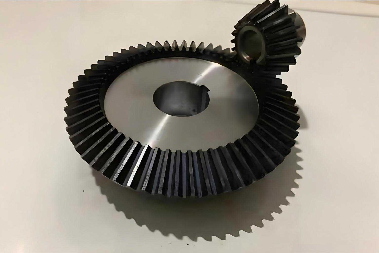
Numerical Example: A Pair of Miter Gears
To demonstrate our method, we analyze a pair of miter gears with an axis angle $\Sigma = 90^\circ$. The primary design parameters are listed in the table below. The remaining blank dimensions are calculated according to AGMA standards.
| Parameter | Pinion | Gear |
|---|---|---|
| Shaft Angle $\Sigma$ [deg] | 90 | |
| Outer Module $m_{et}$ [mm] | 3 | |
| Normal Pressure Angle $\alpha_n$ [deg] | 20 | |
| Number of Teeth $z$ | 20 | 40 |
| Profile Shift Coefficient $x$ | +0.416 | -0.416 |
| Mounting Distance $M_d$ [mm] | 62 | 37 |
In this example, only the pinion tooth surface is modified with longitudinal and profile crowning. The modification effectively transforms the theoretical line contact into a favorable point contact, reducing sensitivity to misalignment.
The Proposed Tooth Contact Analysis Methodology
The core of our new TCA method involves determining the precise contact point for a given pinion rotation angle, calculating the resulting transmission error, and accurately mapping the contact ellipse on the tooth surface, even at its boundaries.
Coordinate Systems and Assembly
The first step in TCA is to represent both gear tooth surfaces in a common static coordinate system $S_s$. For our miter gears, the pinion and gear are assembled on their respective axes, which are perpendicular. The pinion surface $\mathbf{r}_1^{(p)}(u_1, w_1)$ and the gear surface $\mathbf{r}_1^{(g)}(u_2, w_2)$ are transformed into $S_s$ via rotation matrices $\mathbf{M}_{s1}(\phi_1)$ and $\mathbf{M}_{s2}(\phi_2)$, which depend on the rotation angles $\phi_1$ and $\phi_2$:
$$\mathbf{r}_s^{(p)}(u_1, w_1, \phi_1) = \mathbf{M}_{s1}(\phi_1) \cdot \mathbf{r}_1^{(p)}(u_1, w_1)$$
$$\mathbf{r}_s^{(g)}(u_2, w_2, \phi_2) = \mathbf{M}_{s2}(\phi_2) \cdot \mathbf{r}_1^{(g)}(u_2, w_2)$$
Contact Point Determination via the Golden Ratio Method
For a specified pinion rotation angle $\phi_1$, we need to find the corresponding gear rotation angle $\phi_2$ and the surface parameters $(u_1, w_1, u_2, w_2)$ that define the contact point. Conventional methods solve a system of nonlinear equations derived from the condition that the position vectors and surface normals coincide at the contact point. This system can be ill-conditioned.
We propose using the Golden Ratio search algorithm, an optimization technique, to find $\phi_2$. The condition for contact is the coincidence of the position vectors of the two surfaces in the static frame $S_s$:
$$\mathbf{r}_s^{(g)}(u_2, w_2, \phi_2) – \mathbf{r}_s^{(p)}(u_1, w_1, \phi_1) = \mathbf{0}$$
For a fixed $\phi_1$, we search for the $\phi_2$ that minimizes the Euclidean distance between the two surfaces. The search is conducted within a logical interval. For the drive side of a left-hand flank, if $\phi_1$ is less than a reference angle $\alpha$, the gear must rotate clockwise (minimizing $\phi_2$) to achieve contact. If $\phi_1 > \alpha$, the gear must rotate counterclockwise (maximizing $\phi_2$). The Golden Ratio method efficiently finds this minimizing/maximizing $\phi_2$ by iteratively narrowing the search interval based on the golden ratio $\lambda \approx 1.618$. Once $\phi_2$ is found, the corresponding surface parameters that satisfy the distance minimization condition give the contact point coordinates.
Transmission Error Calculation
For perfect conjugate gears with ideal geometry, the gear ratio is constant: $\phi_2 = (z_1 / z_2) \phi_1$. Surface modifications and misalignments cause deviations from this ideal relationship, resulting in transmission error. The transmission error $\Delta \phi_2$ is defined as the deviation of the actual gear angle from its theoretical position:
$$\Delta \phi_2(\phi_1) = \phi_2(\phi_1) – \frac{z_1}{z_2} \phi_1$$
where $\phi_2(\phi_1)$ is the actual gear rotation angle found by the Golden Ratio method for the given $\phi_1$. Plotting $\Delta \phi_2$ against $\phi_1$ shows the function of transmission error. A typical curve for a modified pair of miter gears has a parabolic-like shape within the mesh cycle. The point where the error curve for one tooth pair intersects with the curve for the next tooth pair indicates the potential transfer of load from one pair to the next.
Contact Ellipse Determination via the “Searching Method”
Determining the extent of the contact area is crucial. Instead of approximating an ellipse from principal curvatures, we directly compute the boundary of contact by considering a physical analogy: the imprint left by a marking compound (e.g., Prussian blue) of finite thickness.
At the calculated contact point $\mathbf{p}_c^p$ on the pinion, with unit normal $\mathbf{n}_s^p$, we define a tangent vector $\mathbf{t}_s$ in the common tangent plane:
$$\mathbf{t}_s(u_1, w_1, \phi_1, \theta_c) = \mathbf{t}_{su}^p \cos \theta_c + \mathbf{t}_{sw}^p \sin \theta_c$$
where $\mathbf{t}_{su}^p$ and $\mathbf{t}_{sw}^p$ are orthogonal tangent vectors along the local $u$ and $w$ directions, and $\theta_c$ is an angle parameter sweeping from $0$ to $360^\circ$.
For a given $\theta_c$, the plane defined by $\mathbf{n}_s^p$ and $\mathbf{t}_s$ cuts through both tooth surfaces, creating two intersection curves. We transform a set of sample points from these curves into this 2D cutting plane. A 4th-order B-spline curve is fitted to each set of points. In this plane, the contact condition is modeled by finding the two points on these curves that are simultaneously tangent to a circle with a radius $r_c$ representing the marking compound particle. This leads to a system of equations:
$$x_{po}(u) – x_{go}(v) = 0$$
$$y_{po}(u) – y_{go}(v) = 0$$
where $(x_{po}, y_{po})$ and $(x_{go}, y_{go})$ are the fitted curve equations for the pinion and gear sections in the 2D plane, and $u, v$ are their respective curve parameters. Solving this system for each $\theta_c$ yields a series of boundary points. Transforming these points back to 3D space and connecting them for all $\theta_c$ provides a precise map of the contact pattern boundary on the tooth surface. This method is robust even when the contact area touches the edge of the tooth (boundary contact).
Case Study Results and Validation
We applied both our proposed method and the classic Litvin TCA method to the numerical example of the modified miter gears. The results are compared below.
Contact Path Comparison
The contact path is the locus of contact points on the tooth surface over one mesh cycle. The figure below shows the contact path on the drive side of the gear tooth. The solid line represents the result from Litvin’s method, while the dashed line shows the path calculated by our Golden Ratio-based method. The two paths are virtually identical, confirming the accuracy of our contact point determination algorithm.
Transmission Error Comparison
The transmission error curves are plotted in the following figure. Again, the solid line is from Litvin’s method, and the dashed line is from our proposed method. The excellent agreement between the two curves validates the correctness of our approach for computing the kinematic relationship of the meshing miter gears. The parabolic shape is characteristic of gear pairs with profile modifications.
| Feature | Litvin’s Method | Proposed Method | Agreement |
|---|---|---|---|
| Contact Path Location | Central, slightly biased to toe | Central, slightly biased to toe | Excellent |
| Max Transmission Error [arcsec] | Approx. -12.5 | Approx. -12.7 | Very Good |
| Contact Pattern Shape | Elliptical | Near-Elliptical | Good |
| Boundary Contact Handling | May diverge | Stable and well-defined | Superior in proposed method |
Contact Pattern Comparison
The contact patterns (ellipses) for a specific pinion position are compared. The pattern from Litvin’s method (outline I) is derived from local curvature analysis. The pattern from our searching method (outline II) is derived from the direct boundary calculation described earlier. While both methods predict a similar elongated ellipse oriented along the length of the tooth, our method provides a direct numerical boundary without relying on curvature-based approximation. The close match between the two outlines further reinforces the validity of our overall TCA methodology for analyzing miter gears.
Conclusion
We have successfully developed and demonstrated a new, robust methodology for Tooth Contact Analysis. The method integrates several key techniques: using B-spline surfaces to model modified tooth flanks, employing the Golden Ratio search algorithm to stably locate contact points under all conditions, and introducing a direct “searching method” to determine the precise boundary of the contact pattern by simulating the effect of a finite-thickness marking compound.
The primary advantages of this method are its generality and stability. It is not limited to a specific gear type and performs reliably even in challenging boundary contact scenarios where traditional nonlinear equation solvers may fail. Furthermore, the contact pattern determination is not an approximation based on local curvature but a direct computation of the contact zone boundary, potentially offering higher accuracy, especially for severely misaligned miter gears.
Validation against the established Litvin TCA method for a case study involving modified miter gears showed excellent agreement in the predicted contact path and transmission error, while also producing a consistent contact pattern. This confirms the correctness and practical utility of the proposed approach. This methodology can serve as a powerful tool for the design and performance evaluation of high-precision gear drives, including miter gears, in demanding applications.