
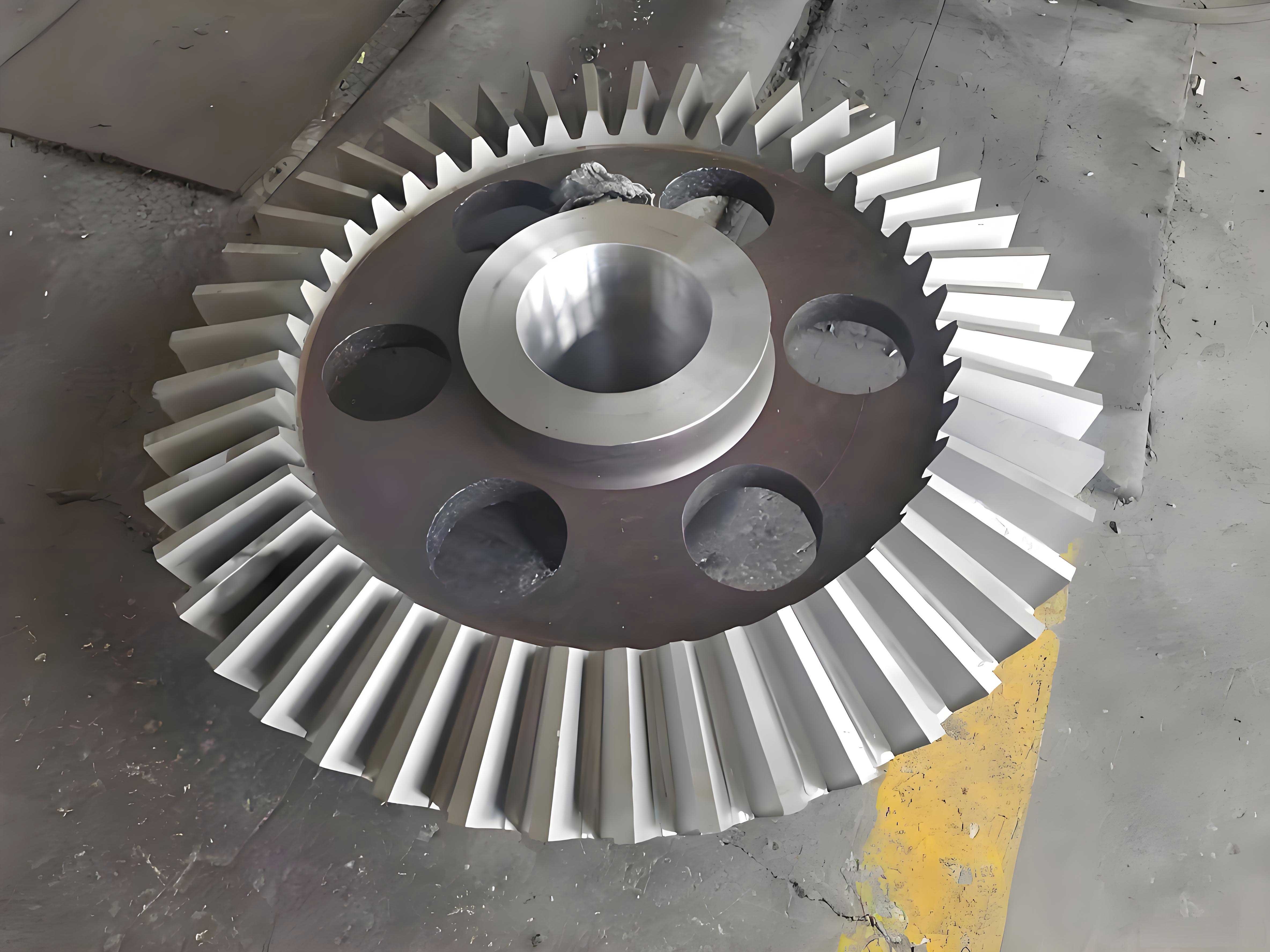
In mechanical transmission systems, miter gears, which are straight bevel gears with a shaft angle of 90 degrees, play a critical role in transferring motion and power between intersecting axes. The performance of these miter gears is heavily influenced by the geometric accuracy of their tooth surfaces, which are complex three-dimensional curves. However, during manufacturing processes such as cutting and subsequent heat treatment, various errors and deformations occur, leading to deviations between the actual machined tooth surfaces and the theoretically designed surfaces. These deviations can adversely affect meshing characteristics, noise, vibration, and fatigue life. Traditional analysis methods often rely on ideal theoretical tooth models, neglecting these real-world imperfections, which may result in inaccurate predictions. To address this, we propose a methodology that integrates actual measured tooth surface data into finite element analysis (FEA) for miter gears. This approach involves measuring the tooth surfaces using precision gear measuring equipment, fitting the measured points with a high-order polynomial to reconstruct a digital tooth surface, and then generating a detailed finite element mesh for static stress analysis. By considering the actual geometry, including manufacturing errors and heat treatment distortions, this method provides a more accurate assessment of the gear’s mechanical behavior under load. The use of miter gears in applications such as automotive differentials, aerospace mechanisms, and industrial machinery underscores the importance of such precise analysis for reliability and performance optimization.
The foundation of this methodology lies in the mathematical representation and fitting of the measured tooth surface points. When a miter gear is manufactured, its tooth surfaces are not perfect; they exhibit variations due to factors like machine tool accuracy, cutter wear, and thermal effects. To capture these variations, we use a gear measuring center, such as a coordinate measuring machine (CMM) specialized for gears, to obtain a set of discrete coordinate points $(x_i, y_i, z_i)$ on the tooth surface, where $i = 1, 2, \ldots, n$. These points reflect the actual geometry after all manufacturing processes. The goal is to construct a continuous digital surface that approximates these points with minimal error. For a smooth surface like that of a miter gear tooth, a polynomial function can serve as an effective approximator. As the polynomial order increases, the approximation error generally decreases, converging to the true surface. We express the tooth surface as a function $z = f(x, y)$, where $z$ is the height coordinate, and $x$ and $y$ are coordinates in the plane perpendicular to the gear axis. The fitting process involves selecting a set of basis functions $\phi_j(x, y)$ that span the polynomial space, and determining coefficients $a_j$ such that the surface $f(x, y) = \sum_{j=1}^{m} a_j \phi_j(x, y)$ best fits the measured points. The quality of fit is evaluated by the sum of squared errors $E(f)$:
$$E(f) = \sum_{i=1}^{n} \left[ z_i – f(x_i, y_i) \right]^2$$
To find the optimal coefficients, we minimize $E(f)$ by setting the partial derivatives with respect to each $a_j$ to zero, leading to a system of linear equations. This system can be solved using numerical methods like Gaussian elimination or least-squares algorithms. The choice of polynomial order is crucial: a low order may not capture surface details, while a very high order might overfit noise. For miter gears, we typically use polynomials up to the fifth order, which balances accuracy and computational efficiency. The fitting error can be quantified as the maximum deviation between the measured points and the fitted surface, often measured in micrometers. This error should be compared to allowable tolerances in gear applications, such as the thickness of marking pastes used in contact pattern tests, which is around 6.35 $\mu$m. By ensuring the fitting error is well below this threshold, we achieve a digital representation that is sufficiently accurate for subsequent analysis.
Once the digital tooth surface is reconstructed, it is essential to analyze its geometric properties, particularly curvature, which influences contact stresses and wear patterns. For a parametric surface $S(u,v)$, where $u$ and $v$ are parameters, the first fundamental form coefficients $E$, $F$, and $G$ describe the metric properties, while the second fundamental form coefficients $L$, $M$, and $N$ describe the curvature. These are defined as:
$$E = \mathbf{S}_u \cdot \mathbf{S}_u, \quad F = \mathbf{S}_u \cdot \mathbf{S}_v, \quad G = \mathbf{S}_v \cdot \mathbf{S}_v$$
$$L = \mathbf{N} \cdot \mathbf{S}_{uu}, \quad M = \mathbf{N} \cdot \mathbf{S}_{uv}, \quad N = \mathbf{N} \cdot \mathbf{S}_{vv}$$
where $\mathbf{S}_u$ and $\mathbf{S}_v$ are partial derivatives, $\mathbf{S}_{uu}$, $\mathbf{S}_{uv}$, and $\mathbf{S}_{vv}$ are second partial derivatives, and $\mathbf{N}$ is the unit normal vector. The normal curvature $k_n$ at a point on the surface in a direction given by the ratio $du:dv$ is expressed as:
$$k_n = \frac{L \, du^2 + 2M \, du \, dv + N \, dv^2}{E \, du^2 + 2F \, du \, dv + G \, dv^2}$$
The principal curvatures $k_1$ and $k_2$ (with $k_1 \leq k_2$) are the extreme values of $k_n$, found by solving the quadratic equation:
$$(EG – F^2) k_n^2 – (EN + GL – 2FM) k_n + (LN – M^2) = 0$$
From these, the Gaussian curvature $K$ and mean curvature $H$ are computed as:
$$K = k_1 k_2, \quad H = \frac{k_1 + k_2}{2}$$
The Gaussian curvature indicates whether the surface is locally elliptic ($K > 0$), hyperbolic ($K < 0$), or parabolic ($K = 0$), which relates to contact conditions in gear meshing. The mean curvature reflects the average bending. For miter gears, analyzing these curvatures helps identify regions of high stress concentration and guides surface modifications like crowning or relief to improve performance.
To demonstrate the application of this methodology, we consider a specific miter gear pair with parameters detailed in Table 1. This gear pair is typical in power transmission systems where right-angle drives are required, and the miter gear design ensures efficient torque transfer with minimal backlash.
| Parameter | Pinion | Gear |
|---|---|---|
| Number of teeth, $Z$ | 16 | 28 |
| Module, $m$ (mm) | 2.5 | 2.5 |
| Pressure angle, $\alpha$ (degrees) | 20 | 20 |
| Shaft angle, $\Gamma$ (degrees) | 90 | 90 |
| Addendum, $h_a$ (mm) | 2.5 | 3 |
| Dedendum, $h_f$ (mm) | 3 | 2.5 |
| Face width, $B$ (mm) | 12.09 | 12.09 |
The tooth surfaces of the miter gear are measured using a high-precision gear measuring center. We collect 45 discrete points on a single tooth flank, ensuring coverage across the entire active profile. These points are then subjected to polynomial fitting. To determine the appropriate polynomial order, we compute the maximum fitting error for different orders, as shown in Table 2. The error decreases significantly with increasing order, and the fifth-order polynomial yields a maximum error of only 0.314 $\mu$m, which is well below the 6.35 $\mu$m threshold, making it suitable for accurate analysis of miter gears.
| Polynomial Order | Maximum Error ($\mu$m) |
|---|---|
| Third-order | 32.8 |
| Fourth-order | 3.361 |
| Fifth-order | 0.314 |
The coefficients for the fifth-order polynomial, which has 21 terms to fully represent a bivariate surface, are listed in Table 3. The polynomial takes the form:
$$z = a_0 + a_1 x + a_2 y + a_3 x^2 + a_4 x y + a_5 y^2 + a_6 x^3 + a_7 x^2 y + a_8 x y^2 + a_9 y^3 + a_{10} x^4 + a_{11} x^3 y + a_{12} x^2 y^2 + a_{13} x y^3 + a_{14} y^4 + a_{15} x^5 + a_{16} x^4 y + a_{17} x^3 y^2 + a_{18} x^2 y^3 + a_{19} x y^4 + a_{20} y^5$$
| Coefficient | Value |
|---|---|
| $a_0$ | -79.1636 |
| $a_1$ | -3.2171 |
| $a_2$ | -1.8177 |
| $a_3$ | 0.0846 |
| $a_4$ | 0.0554 |
| $a_5$ | -0.0248 |
| $a_6$ | -0.0011 |
| $a_7$ | 0.0005 |
| $a_8$ | -0.0017 |
| $a_9$ | 0.0010 |
| $a_{10}$ | 0.000079 |
| $a_{11}$ | 0.00000049 |
| $a_{12}$ | -0.00001275 |
| $a_{13}$ | 0.00002023 |
| $a_{14}$ | -0.00001174 |
| $a_{15}$ | -0.00000002 |
| $a_{16}$ | -0.00000000 |
| $a_{17}$ | -0.00000001 |
| $a_{18}$ | 0.00000000 |
| $a_{19}$ | -0.00000008 |
| $a_{20}$ | 0.00000004 |
After fitting, we ensure the correct tooth thickness for the miter gear by controlling the rotation of the fitted surface. The reference point is the midpoint on the pitch cone, where the coordinate $y$ is set to zero. By solving the fitting equation at this point, we adjust the rotation angle $\phi$ so that points on the pitch cone from both flanks coincide. Then, rotating the surface by an angle of $\pi / Z$ generates the full tooth thickness, ensuring the geometric integrity of the miter gear model. This step is critical because inaccurate tooth thickness can lead to improper meshing and increased stresses.
With the digital tooth surface defined, we proceed to finite element mesh generation. For accuracy, we employ mapping grid techniques, which involve projecting the parametric surface onto a regular grid in the parameter domain and then mapping it back to the physical space. This approach produces a structured mesh of hexahedral elements, which are advantageous for stress analysis due to their superior performance in capturing stress gradients. The element type selected is SOLID45, an eight-node hexahedral element commonly used in structural mechanics. The material properties for the miter gear, typically made of alloy steel, are listed in Table 4. These properties are essential for simulating the linear elastic behavior under static loads.
| Property | Value |
|---|---|
| Elastic modulus, $E$ (GPa) | 210 |
| Poisson’s ratio, $\nu$ | 0.3 |
| Density, $\rho$ (kg/m³) | 7800 |
The finite element model is constructed in ANSYS software. To reduce computational expense while capturing the essential meshing behavior, we model only three teeth of the miter gear, as only a few teeth are in contact at any given time. The mesh is refined along the tooth profile and root region, where stress concentrations are expected. The nodes on the gear’s bottom surface and symmetric planes are fully constrained (all degrees of freedom fixed) to simulate the mounting conditions. This boundary condition ensures that the gear is stationary, allowing us to apply loads and observe deformations realistically.
Loading is applied to simulate the worst-case bending stress scenario, which occurs when a single tooth pair is in contact at the highest point of single tooth contact. For simplicity, we apply a concentrated force at the tooth tip in the direction of the normal pressure angle (20 degrees). The magnitude of the force is based on the rated torque for the miter gear application. Although actual gear contact involves distributed loads along the tooth flank, this simplified loading provides a conservative estimate of bending stresses and is commonly used in preliminary analyses. The applied force $F$ can be calculated from the torque $T$ and pitch radius $r$ as $F = T / r$, but for this study, we assume a nominal load to illustrate the method.
The finite element analysis yields stress and deformation results. The equivalent (von Mises) stress distribution shows that the maximum stress occurs at the point of load application on the tooth tip, with significant stress concentrations at the tooth root due to bending. The deformation pattern indicates that the tooth deflects under load, with the tip experiencing the largest displacement. These results are consistent with classical beam theory for gear teeth but provide more detailed insights due to the precise geometry of the miter gear. For instance, the stress at the tooth root, a critical location for fatigue failure, can be extracted and compared to allowable material limits. Additionally, the curvature analysis from earlier can correlate with stress patterns; regions with high Gaussian curvature may exhibit higher contact stresses if involved in meshing.
To quantify the results, we summarize key outputs in Table 5. These values are indicative and would vary with load magnitude and gear dimensions, but they demonstrate the capability of the method to provide precise data for miter gear design evaluation.
| Output Parameter | Value |
|---|---|
| Maximum equivalent stress (MPa) | 285.6 |
| Maximum deformation at tooth tip (mm) | 0.0123 |
| Tooth root bending stress (MPa) | 210.4 |
| Stress concentration factor at root | 1.85 |
The analysis reveals that the miter gear tooth experiences bending stresses that are within typical safe limits for alloy steel, but the stress concentration at the root highlights the need for fillet optimization. Furthermore, the deformation suggests that under higher loads, contact misalignment might occur, emphasizing the importance of surface modifications like crowning. By using the measured tooth surface, we account for actual manufacturing errors that could exacerbate these issues, providing a more reliable assessment than theoretical models.
In conclusion, the integration of measured tooth surface data into finite element analysis for miter gears offers a robust approach to performance evaluation. The use of high-order polynomial fitting, with fifth-order proving sufficient, allows accurate digital reconstruction of the tooth geometry, capturing manufacturing-induced deviations. The curvature analysis provides insights into surface topology, aiding in contact mechanics understanding. The finite element model, built via mapping mesh techniques, enables detailed static stress analysis, revealing critical stress regions and deformation patterns. This methodology is particularly valuable for miter gears, where precise right-angle transmission is crucial, and small geometric errors can lead to significant performance degradation. Future work could extend this approach to dynamic analysis, thermal effects, or fatigue life prediction, further enhancing the design and reliability of miter gears in demanding applications. Overall, by bridging the gap between theoretical design and actual manufacturing, this method supports the development of more durable and efficient miter gear systems.