
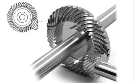
The design and manufacture of high-performance spiral bevel gears are critical for advanced power transmission systems in aerospace, automotive, and marine applications. These gears are prized for their smooth operation, high load-carrying capacity, and low noise characteristics. A central challenge in their design is the precise control of the contact pattern—the area on the tooth flank where mating teeth make contact under load. The orientation of this contact path, often characterized by its bias angle, is a fundamental design parameter that directly influences gear performance, including load distribution, stress conditions, and sensitivity to misalignment. Achieving a prescribed bias angle is therefore a primary objective in the active design of spiral bevel gears.
Traditionally, gear design relied on iterative trial-and-error methods, such as the local conjugation approach, which required extensive physical testing and adjustment. A significant advancement came with the development of the local synthesis method, which allows for the predefinition of meshing performance characteristics at a designated reference point on the tooth surface. This method enables the active design of spiral bevel gears by directly calculating machine-tool settings based on desired contact conditions. However, a practical complication arises because the design specification for the contact path orientation is typically given in a projected plane (like a blueprint or inspection chart), while the local synthesis method operates with parameters defined on the three-dimensional tooth surface. The bias angle observed in the projection plane is not equal to the angle on the actual tooth surface due to the effects of the coordinate transformation involved in projection. This discrepancy necessitates an active and precise design methodology to bridge the gap between the specified target in the projection and the necessary input for the synthesis algorithm.
This article presents a comprehensive, integrated methodology for the active design of the bias angle of the contact path in spiral bevel gears. The approach synergistically combines the local synthesis method for initial parameter generation, Tooth Contact Analysis (TCA) for simulation and verification, and an unconstrained optimization routine to iteratively refine the design until the projected bias angle matches the target value. The core of the method involves adjusting the input bias angle for the local synthesis process based on feedback from TCA performed in the projection plane. A key finding is that the input angle for synthesis must be deliberately set lower than the desired final angle in the projection. The entire process is automated, ensuring accuracy and efficiency, and is demonstrated through a detailed case study.
1. Methodology for Active Bias Angle Design
The proposed active design flow is a closed-loop process. It begins with a target specification, uses analytical tools to generate and evaluate a design, and employs optimization to correct deviations. The primary goal is to determine the correct bias angle parameter, denoted as $\eta_2$, which must be supplied to the local synthesis algorithm so that, after machining and projection, the gear pair exhibits the desired bias angle $\eta’_2$ in the projected view.
1.1 The Bias Angle Discrepancy: Tooth Surface vs. Projection Plane
Consider the mean contact point $M$ on the tooth surface of a spiral bevel gear. On the tangent plane at $M$, the contact path has a certain direction. The angle between the tangent to the contact path ($\overrightarrow{mn}$) and the root line (or a cone generator) is the surface bias angle $\eta_2$.
For design and inspection purposes, the three-dimensional tooth surface is often projected onto a plane, typically using a transformation that maps coordinates $(x, y, z)$ to $(X, R)$, where $x$ is along the gear axis, and $R$ is the radial distance:
$$X = x, \quad R = \sqrt{y^2 + z^2}.$$
This projection is not isometric; it distorts angles. Consequently, the bias angle $\eta’_2$ measured in the projected plane $(X, R)$ is always greater than the true surface angle $\eta_2$.
$$\eta’_2 > \eta_2.$$
The relationship is governed by the geometry of the projection. Therefore, to achieve a target projected angle $\eta’_{2\text{target}}$, the designer must purposefully choose a smaller value for $\eta_2$ as input to the synthesis. The exact value of $\eta_2$ required is not straightforward and forms the crux of the optimization problem.
1.2 Initial Design via Local Synthesis
The local synthesis method is the starting point for generating the machine-tool settings for the pinion. The process follows these steps:
- Gear Blank and Basic Machine Settings: The geometric parameters of the gear blank (number of teeth, shaft angle, spiral angle, etc.) and the machine settings for generating the gear (cutter radius, cutter blade angle, machine root angle, etc.) are defined first.
- Gear Tooth Surface Calculation: The gear tooth surface geometry at the mean point $M$ is calculated based on its manufacturing parameters.
- Pinion Synthesis Input: At point $M$, along with the known gear surface, the following meshing characteristics are prescribed for the pinion:
- The derivative of the transmission error function (controlling the shape of the transmission error curve).
- The desired bias angle on the tooth surface, $\eta_{2l}$.
- The ratio of the contact ellipse axes (controlling the shape of the contact pattern).
- Calculation of Pinion Machine Settings: The local synthesis equations are solved to determine the pinion tooth surface geometry at $M$ that satisfies the prescribed conditions in a differential neighborhood around the point. This geometry is then converted into the corresponding machine-tool settings (modified cutter blade angle, machine root angle, ratio of roll, etc.).
A critical adjustment is made before inputting the bias angle into synthesis. The required input $\eta_{2l}$ is not simply the target surface angle $\eta_2$, but must account for the orientation of the generating tool relative to the gear’s principal directions. The corrected input is:
$$\eta_{2l} = \eta_2 + \theta^{(2,cr2)}.$$
Here, $\theta^{(2,cr2)}$ is the angle between the principal direction of the gear surface and the principal direction of the generating cradle. This angle is calculated from the gear surface’s principal curvatures and the kinematic relationship between the gear and the cutter. Its tangent is given by:
$$\tan 2\theta^{(2,cr2)} = \frac{2a_{13}a_{23}}{a_{23}^2 – a_{13}^2 + (k_{e1^{(2)}}^{(2)} – k_{e2^{(2)}}^{(2)}) a_{33}}.$$
The coefficients $a_{ij}$ are complex functions of the principal curvatures $k_{e1^{(i)}}^{(i)}$, the relative velocity vectors $\mathbf{v}^{(12)}$, and the angular velocities $\boldsymbol{\omega}^{(i)}$ of the mating surfaces at point $M$.
1.3 Verification and Analysis via Tooth Contact Analysis (TCA)
The machine settings obtained from local synthesis must be rigorously verified. This is done through numerical Tooth Contact Analysis (TCA). TCA simulates the meshing of the theoretically generated pinion and gear tooth surfaces. The fundamental condition for continuous tangency is expressed by a system of vector equations:
$$
\begin{aligned}
\mathbf{r}_h^{(1)}(\theta_p, \phi_{cr1}, \phi_1) &= \mathbf{r}_h^{(2)}(\theta_g, \phi_{cr2}, \phi_2), \\[4pt]
\mathbf{n}_h^{(1)}(\theta_p, \phi_{cr1}, \phi_1) &= \mathbf{n}_h^{(2)}(\theta_g, \phi_{cr2}, \phi_2).
\end{aligned}
$$
Where:
- $\mathbf{r}_h^{(i)}$ is the position vector of a point on tooth surface $i$ ($i=1$ for pinion, $i=2$ for gear) in the fixed housing coordinate system $S_h$.
- $\mathbf{n}_h^{(i)}$ is the unit normal vector at that point.
- $\theta_p, \phi_{cr1}$ and $\theta_g, \phi_{cr2}$ are the surface parameters defining a point on the pinion and gear tooth surfaces, respectively.
- $\phi_1$ and $\phi_2$ are the rotation angles of the pinion and gear.
By solving this system for a sequence of pinion rotation angles $\phi_1$, the corresponding gear angles $\phi_2$ and the contact points on both tooth surfaces are determined. The results are:
- Transmission Error (TE) Curve: $\Delta \phi_2 = \phi_2 – (N_1/N_2)\phi_1$, where $N_1$ and $N_2$ are the tooth numbers. A low-amplitude, parabolic TE curve is often a design goal for low noise.
- Contact Path: The locus of contact points on the tooth surface, typically visualized in the projection plane $(X, R)$.
The TCA output provides the actual projected bias angle $\eta’_{2\text{sim}}$ from the simulated contact path. This is compared to the target $\eta’_{2\text{target}}$.
1.4 Optimization Loop for Bias Angle Correction
Since the first attempt (using $\eta_2 = \eta’_{2\text{target}}$) will yield $\eta’_{2\text{sim}} > \eta’_{2\text{target}}$, an optimization loop is employed to find the correct $\eta_2$. The process is automated as follows:
- Initialization: Set the target projected angle $\eta’_{2\text{target}}$. Set the initial guess for the synthesis input angle, often $\eta_2^{(0)} = \eta’_{2\text{target}}$.
- Local Synthesis: Use $\eta_2^{(k)}$ (angle for iteration $k$) to calculate the corrected input $\eta_{2l}$ and run the local synthesis to obtain pinion machine settings.
- TCA Simulation: Perform TCA with the new pinion and the fixed gear settings.
- Angle Extraction: From the TCA contact path in the $(X, R)$ plane, fit a line through points near the mean contact point $M’$ (the projection of $M$) and calculate the simulated projected bias angle $\eta’_{2\text{sim}}^{(k)}$.
- Objective Function Evaluation: Define the error as $F(\eta_2) = | \eta’_{2\text{sim}}(\eta_2) – \eta’_{2\text{target}} |$.
- Optimization Step: Use an unconstrained optimization algorithm (e.g., Nelder-Mead, gradient-based) to adjust $\eta_2$ to minimize $F(\eta_2)$. The updated value $\eta_2^{(k+1)}$ is fed back to step 2.
- Convergence: The loop terminates when $F(\eta_2)$ is below a specified tolerance, meaning the simulated contact path in projection aligns with the desired direction.
The following flowchart summarizes the integrated active design methodology:
[Target: η'₂_target] → [Set Initial η₂] → [Local Synthesis (with η₂l=η₂+θ)] → [Calculate Pinion Settings]
                                                                 |
                                                                 V
[Converged?] ← [Optimization Algorithm] ← [Extract η'₂_sim] ← [TCA Simulation]
    |                                                                 ^
    V                                                                 |
[Final Design] -------------------------------------------------------
2. Theoretical Framework and Key Equations
The methodology is underpinned by the mathematical theory of gearing. Key equations are summarized below.
2.1 Local Synthesis Equations
The local synthesis ensures second-order contact between the pinion and gear tooth surfaces at point $M$. It involves solving for the pinion surface’s second-order parameters (principal curvatures and directions) based on the known gear surface and the prescribed kinematics. The core conditions relate the relative normal curvatures and the relative torsion along the contact path direction. The equation involving the bias angle $\eta_2$ is embedded in the definition of the direction vector $\mathbf{e}_t^{(2)}$ tangent to the contact path on the gear surface:
$$\mathbf{e}_t^{(2)} = \mathbf{e}_1^{(2)} \cos \eta_2 + \mathbf{e}_2^{(2)} \sin \eta_2,$$
where $\mathbf{e}_1^{(2)}, \mathbf{e}_2^{(2)}$ are the principal direction vectors of the gear surface at $M$. The synthesis algorithm then ensures that the following equation holds, which governs the length and orientation of the instantaneous contact ellipse:
$$ \kappa_\Sigma = \kappa^{(1)} – \kappa^{(2)} = \frac{1}{a^2}.$$
Here, $\kappa_\Sigma$ is the normal relative curvature in the direction perpendicular to $\mathbf{e}_t^{(2)}$, $\kappa^{(i)}$ are the normal curvatures of the pinion and gear, and $a$ is the semi-major axis of the contact ellipse, which is prescribed.
2.2 Tooth Contact Analysis (TCA) System
The TCA system, as stated earlier, consists of five independent scalar equations derived from the two vector equations. For a given pinion rotation $\phi_1$, we solve for the five unknowns: $\theta_p$, $\phi_{cr1}$, $\theta_g$, $\phi_{cr2}$, and $\phi_2$.
$$
\begin{cases}
f_1(\theta_p, \phi_{cr1}, \theta_g, \phi_{cr2}, \phi_2; \phi_1) = 0,\\
f_2(\theta_p, \phi_{cr1}, \theta_g, \phi_{cr2}, \phi_2; \phi_1) = 0,\\
f_3(\theta_p, \phi_{cr1}, \theta_g, \phi_{cr2}, \phi_2; \phi_1) = 0,\\
f_4(\theta_p, \phi_{cr1}, \theta_g, \phi_{cr2}, \phi_2; \phi_1) = 0,\\
f_5(\theta_p, \phi_{cr1}, \theta_g, \phi_{cr2}, \phi_2; \phi_1) = 0.
\end{cases}
$$
This nonlinear system is typically solved using the Newton-Raphson method. The solution trace for a range of $\phi_1$ values defines the contact path and the function $\phi_2(\phi_1)$, from which the transmission error is computed.
2.3 Projection and Angle Calculation
Once the contact points $\mathbf{r}_h = [x_h, y_h, z_h]^T$ are found via TCA, they are projected onto the $(X, R)$ plane for analysis:
$$ X = x_h, \quad R = \sqrt{y_h^2 + z_h^2}.$$
A set of $n$ points $(X_i, R_i)$ near the mean point $M’$ are used to fit a straight line $R = mX + b$ using the least-squares method. The fitted slope $m$ is related to the projected bias angle $\eta’_2$. If the root line in projection is along the $X$-axis, then:
$$ \eta’_2 = \arctan(m).$$
This calculated angle is the value $\eta’_{2\text{sim}}$ used in the optimization objective function.
3. Implementation and Case Study
To demonstrate the effectiveness of the active design method for controlling the bias angle in spiral bevel gears, a detailed case study is presented. The gear pair is designed for a high-performance application requiring precise contact pattern control.
3.1 Initial Gear Pair Data and Target
The basic geometric parameters of the spiral bevel gear pair are listed in the table below. The design aims for a smooth, localized contact pattern with a specific orientation.
| Parameter | Pinion | Gear |
|---|---|---|
| Number of Teeth | 38 | 43 |
| Shaft Angle | 90° | |
| Pressure Angle | 20° | |
| Mean Spiral Angle | 35° | |
| Hand of Spiral | Left Hand | Right Hand |
| Outer Cone Distance | 52.507 mm | |
| Face Width | 6.7 mm | |
| Whole Depth | 3.455 mm | |
The machine settings for generating the gear member are fixed and shown in the following table. These are standard settings derived from the gear blank geometry.
| Parameter | Value |
|---|---|
| Cutter Blade Angle | 21.1667° |
| Cutter Radius | 88.9 mm |
| Point Width | 0.9381 mm |
| Radial Setting | 43.4093 mm |
| Basic Machine Root Angle | 46.6259° |
The target performance parameters for the local synthesis of the pinion are set as follows. The key active design target is the projected bias angle.
| Parameter | Target Value |
|---|---|
| First Derivative of Transmission Error | 0.01 |
| Target Projected Bias Angle ($\eta’_{2\text{target}}$) | 35° |
| Contact Ellipse Axis Ratio (Semi-minor / Semi-major) | 0.2 |
3.2 Initial Design Attempt and Problem Identification
For the first iteration, the synthesis input surface bias angle was naively set equal to the target: $\eta_2^{(0)} = 35°$. After applying the local synthesis correction ($\eta_{2l} = \eta_2^{(0)} + \theta^{(2,cr2)}$), the pinion machine settings were calculated. TCA was then performed with these settings.
The resulting contact path was projected onto the $(X, R)$ plane. A line was fitted through the points near the mean contact point $M’$. The slope of this line indicated a simulated projected bias angle of $\eta’_{2\text{sim}}^{(0)} = 42.759°$. This was a significant deviation of +7.759° from the target of 35°. The contact path, though smooth, was oriented at a much steeper angle than desired. This clearly demonstrated the necessity of the active correction loop. The transmission error curve from this initial design was parabolic and of low amplitude, indicating good kinematic performance, but the contact location was incorrect.
3.3 Active Optimization Process and Results
The optimization algorithm was initiated with the objective to minimize $F(\eta_2) = | \eta’_{2\text{sim}}(\eta_2) – 35° |$. The algorithm systematically adjusted the input $\eta_2$ for local synthesis. After several iterations, convergence was achieved.
The final, optimized value for the surface bias angle input to local synthesis was found to be:
$$\eta_2^{\text{(optimal)}} = 28.974°.$$
This confirms the theoretical premise: to achieve a projected angle of 35°, the synthesis must be performed with a surface angle approximately 6° smaller.
The key machine-tool settings for the pinion, comparing the initial (incorrect) guess and the final optimized design, are summarized below. Notable changes occurred in parameters like the radial setting and the machine root angle to achieve the corrected tooth surface geometry.
| Parameter | Initial Design ($\eta_2=35°$) | Optimized Design ($\eta_2=28.974°$) |
|---|---|---|
| Modified Cutter Blade Angle | 18.8333° | 18.8333° |
| Tool Point Radius | 62.216 mm | 61.438 mm |
| Radial Setting | 55.442 mm | 53.899 mm |
| Machine Root Angle | 39.5258° | Adjusted (via ratio) |
| Ratio of Roll | 1.773 | 1.766 |
The final TCA results using the optimized settings are outstanding:
- Projected Bias Angle: $\eta’_{2\text{sim}}^{\text{(final)}} = 35.002°$. The contact path in the projection plane is now virtually perfectly aligned with the 35° target line.
- Transmission Error: The TE curve remains a smooth, low-amplitude parabolic function. Crucially, its shape and amplitude did not distort during the optimization process for the bias angle. This indicates that the bias angle and the transmission error characteristics can be controlled independently through local synthesis, which is a significant advantage of the method.
- Contact Ellipse: The size and shape of the contact ellipse at the mean point conform to the prescribed axis ratio, ensuring a stable and favorable load distribution.
4. Discussion and Design Implications
The successful case study validates the integrated active design methodology. Several important conclusions and practical implications can be drawn for the design of spiral bevel gears:
4.1 The Necessity of Active, Compensated Design
The discrepancy between the surface bias angle $\eta_2$ and the projected bias angle $\eta’_2$ is systematic and non-negligible. Assuming they are equal will lead to a design error on the order of several degrees, as shown in the example. For high-precision applications common in aerospace and other demanding fields, such an error is unacceptable. The presented method provides a deterministic, computational path to compensate for this geometric effect, moving from iterative “cut-and-try” to a predictive, first-pass-correct design philosophy.
4.2 Independence of Bias Angle and Transmission Error Control
A critical finding from the optimization process is that adjusting the input $\eta_2$ to achieve the target projected contact path direction did not alter the fundamental parabolic shape of the transmission error curve. This is a direct consequence of the structure of the local synthesis equations. The transmission error function (its value, first derivative, and second derivative at $M$) and the bias angle $\eta_2$ are independent parameters that can be prescribed separately. This decoupling allows the designer to optimize for low noise (via parabolic TE) and optimal load-carrying capacity or misalignment tolerance (via bias angle) simultaneously without compromise.
4.3 Practical Design Rule
The study concretely establishes a practical design rule: The bias angle parameter used as input for the local synthesis of spiral bevel gears must be intentionally set to a value less than the desired bias angle in the rotational axis projection plane. The magnitude of the required reduction ($\Delta \eta = \eta’_{2\text{target}} – \eta_2^{\text{optimal}}$) is not constant; it depends on the specific gear geometry, spiral angle, and pressure angle. Therefore, the automated optimization loop described is the most robust way to determine the correct value for any given gear set.
4.4 Extension to Other Contact Parameters
While this article focuses on the active design of the bias angle, the same methodological framework—local synthesis + TCA verification + optimization—is directly applicable to other contact characteristics. For instance, one could actively design for a specific contact ellipse size (semi-major axis length) or a specific second-order (curvature) of the transmission error curve. The objective function in the optimization loop would simply be modified accordingly (e.g., $F = |a_{\text{sim}} – a_{\text{target}}|$). This makes the approach a versatile platform for the comprehensive multi-objective optimization of spiral bevel gear meshing performance.
5. Conclusion
This article has presented a complete and effective methodology for the active design of the contact path bias angle in spiral bevel gears. The method integrates the analytical power of local synthesis, the verification capability of numerical Tooth Contact Analysis, and the precision of modern optimization algorithms into a seamless digital workflow. The core challenge addressed is the transformation difference between the three-dimensional tooth surface geometry and the two-dimensional projection plane used for specification and inspection.
The key results from the implementation and case study are:
- The bias angle parameter input to the local synthesis process ($\eta_2$) must be less than the target angle specified in the projection drawing ($\eta’_2$). An optimization routine is necessary to find the correct compensating value.
- The control of the bias angle is effectively decoupled from the control of the transmission error curve. Optimizing for the desired contact path orientation does not compromise the low-noise, parabolic transmission error characteristic, enabling simultaneous optimization of multiple performance metrics.
- The proposed active design process is automated, reliable, and eliminates the need for physical trial-and-error, leading to faster development cycles and higher precision in the manufacture of advanced spiral bevel gears.
This methodology represents a significant step forward in the digital design and manufacturing of high-performance gear drives. It provides engineers with a powerful tool to proactively and accurately dictate critical meshing behavior, ultimately contributing to more efficient, reliable, and quieter power transmission systems in aerospace and other high-technology industries. Future work may involve extending the optimization to include robustness against misalignments or integrating the process with stress analysis for simultaneous durability optimization.