
The pursuit of optimal power transmission in modern machinery places stringent demands on gear performance. Among various gear types, spiral bevel gears are pivotal components in systems requiring efficient, high-torque, and non-parallel shaft power transfer, such as automotive differentials, helicopter transmissions, and heavy industrial equipment. The core challenge in their application lies in ensuring superior meshing quality, characterized by a controlled contact pattern and minimal transmission error. This directly influences noise, vibration, durability, and overall system reliability. Traditional methods for evaluating spiral bevel gear meshing involve physical testing on roll testers, which is time-consuming, costly, and offers limited predictive capability for design variations. Therefore, a robust, computational methodology is essential for the design and analysis phase.
Tooth Contact Analysis (TCA) has emerged as the fundamental computational technique to address this need. TCA simulates the meshing of conjugate or mismatched gear tooth surfaces under unloaded or lightly loaded conditions. It calculates the path of contact across the tooth flank and the resulting transmission error throughout the mesh cycle. This simulation effectively predicts the contact ellipse (or pattern) location, shape, and orientation, as well as the motion transmission characteristics, before physical prototypes are manufactured. This article details the comprehensive process of building a TCA simulation model for spiral bevel gears, with a specific focus on implementation using MATLAB. The mathematical formulation, solution strategy, and practical analysis of results are presented to provide a valuable tool for engineers and researchers aiming to enhance spiral bevel gear design accuracy and efficiency.
Mathematical Modeling of Spiral Bevel Gear Tooth Surfaces
The geometry of a spiral bevel gear tooth is complex, generated by the relative motion between a cutting tool (cutter head) and the gear blank on a specific machine tool. Different machine-tool systems (e.g., Gleason, Klingelnberg, Oerlikon) employ distinct generation principles, leading to variations in the final tooth surface equation. This work adopts the widely used Gleason system for derivation. The core principle involves defining the cutter surface in its local coordinate system and then transforming it into the coordinate system of the finished gear through a series of rotational and translational transformations that replicate the machine settings.
Cutter Surface and Coordinate Systems
The generating surface for the gear tooth is typically the surface of the cutting blades on the cutter head. For spiral bevel gears, this is often a conical surface (for single-sided methods) or a combination of convex and concave surfaces. We first establish the necessary coordinate systems.
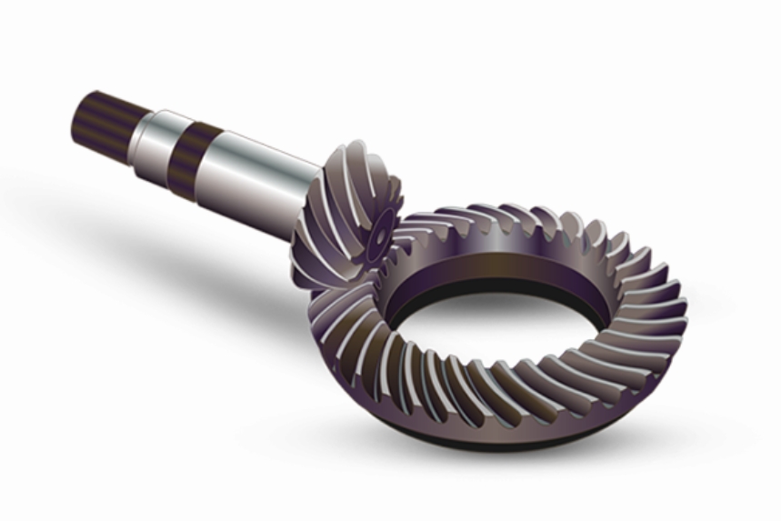
For the gear (wheel), the following coordinate systems are defined, as conceptually illustrated in related machine tool diagrams:
- $S_e(X_e, Y_e, Z_e)$: Attached to the cutter head. Origin $O_e$ at the cutter center. The $X_eO_eY_e$ plane is typically the cutter face plane.
- $S_g(X_g, Y_g, Z_g)$: Attached to the generating gear (cradle).
- $S_m(X_m, Y_m, Z_m)$: Attached to the machine column.
- $S_a(X_a, Y_a, Z_a)$: An auxiliary system.
- $S_2(X_2, Y_2, Z_2)$: Attached to the finished gear, rotating with it.
The cutter surface, represented in $S_e$, is a cone. Its position vector $\vec{r}^{(e)}$ and unit normal vector $\vec{n}^{(e)}$ can be parameterized by two surface coordinates: the radial distance $u_G$ and the rotational angle $\theta_G$ (or a related parameter). For a straight-sided blade with profile angle $\alpha_G$, the equations are:
$$
\begin{align}
\vec{r}^{(e)}(u_G, \theta_G) &= \begin{bmatrix}
(r_G \pm u_G \sin\alpha_G) \cos\theta_G \\
(r_G \pm u_G \sin\alpha_G) \sin\theta_G \\
\mp u_G \cos\alpha_G \\
1
\end{bmatrix}, \\
\vec{n}^{(e)}(\theta_G) &= \begin{bmatrix}
\cos\alpha_G \cos\theta_G \\
\cos\alpha_G \sin\theta_G \\
\pm \sin\alpha_G \\
0
\end{bmatrix}.
\end{align}
$$
where $r_G$ is the cutter point radius, and the $\pm$ signs correspond to convex and concave sides, respectively. The homogeneous coordinate representation is used for easier transformation.
Tooth Surface of the Gear (Wheel)
The gear tooth surface is generated by enveloping the cutter surface as the cradle rotates. The transformation from the cutter system $S_e$ to the gear system $S_2$ involves several steps: $S_e \to S_g \to S_m \to S_a \to S_2$. Each step is represented by a homogeneous coordinate transformation matrix $\mathbf{M}$.
The surface point and normal in the gear coordinate system $S_2$ are obtained by successive transformations:
$$
\begin{align}
\vec{r}^{(2)}(u_G, \theta_G, \phi_2) &= \mathbf{M}_{2a}(\phi_2) \cdot \mathbf{M}_{am} \cdot \mathbf{M}_{mg} \cdot \mathbf{M}_{ge}(\theta_G) \cdot \vec{r}^{(e)}(u_G, \theta_G), \\
\vec{n}^{(2)}(\theta_G, \phi_2) &= \mathbf{L}_{2a}(\phi_2) \cdot \mathbf{L}_{am} \cdot \mathbf{L}_{mg} \cdot \mathbf{L}_{ge}(\theta_G) \cdot \vec{n}^{(e)}(\theta_G).
\end{align}
$$
Here, $\phi_2$ is the rotation angle of the gear blank during generation. $\mathbf{M}_{ij}$ are 4×4 homogeneous transformation matrices, and $\mathbf{L}_{ij}$ are the 3×3 rotational submatrices extracted from the corresponding $\mathbf{M}_{ij}$. The matrices incorporate machine settings such as cradle angle $q$, machine root angle $\gamma_m$, sliding base $X_B$, blank offset $E_m$, and the ratio of roll between the cradle and the gear blank. The explicit forms of these matrices are defined by the spatial geometry of the machine tool. The resulting vector function $\vec{r}^{(2)}(u_G, \theta_G, \phi_2)$ represents the family of cutter surfaces in $S_2$. The specific envelope, which is the gear tooth surface, satisfies the equation of meshing between the cutter and the generating gear:
$$
f_G(u_G, \theta_G, \phi_2) = \vec{n}^{(g)} \cdot \vec{v}^{(ge)} = 0.
$$
$\vec{n}^{(g)}$ is the cutter normal expressed in the generating gear system $S_g$, and $\vec{v}^{(ge)}$ is the relative velocity between the cutter and the generating gear. Solving this equation allows the elimination of one parameter, typically expressing $\phi_2$ as a function of $u_G$ and $\theta_G$, or vice versa. The final gear tooth surface $\vec{R}^{(2)}$ can be expressed with two independent parameters (e.g., $\theta_G$ and $u_G$), with $\phi_2$ implicitly defined by the equation of meshing $f_G=0$.
Tooth Surface of the Pinion
The derivation for the pinion tooth surface follows an analogous procedure but with its own set of machine settings and coordinate systems ($S_f$ for pinion cutter, $S_1$ for finished pinion). The pinion is often cut with a modified process (e.g., modified roll) to localize bearing contact. The pinion cutter surface equations in $S_f$ are similar, parameterized by $u_P$ and $\theta_P$ with a profile angle $\alpha_P$:
$$
\begin{align}
\vec{r}^{(f)}(u_P, \theta_P) &= \begin{bmatrix}
(r_P \pm u_P \sin\alpha_P) \cos\theta_P \\
(r_P \pm u_P \sin\alpha_P) \sin\theta_P \\
\mp u_P \cos\alpha_P \\
1
\end{bmatrix}, \\
\vec{n}^{(f)}(\theta_P) &= \begin{bmatrix}
\cos\alpha_P \cos\theta_P \\
\cos\alpha_P \sin\theta_P \\
\pm \sin\alpha_P \\
0
\end{bmatrix}.
\end{align}
$$
The transformation chain from $S_f$ to the pinion coordinate system $S_1$ involves its own sequence: $S_f \to S_p \to S_n \to S_b \to S_1$. The pinion tooth surface in $S_1$ is given by:
$$
\begin{align}
\vec{r}^{(1)}(u_P, \theta_P, \phi_1) &= \mathbf{M}_{1b}(\phi_1) \cdot \mathbf{M}_{bn} \cdot \mathbf{M}_{np} \cdot \mathbf{M}_{pf}(\theta_P) \cdot \vec{r}^{(f)}(u_P, \theta_P), \\
\vec{n}^{(1)}(\theta_P, \phi_1) &= \mathbf{L}_{1b}(\phi_1) \cdot \mathbf{L}_{bn} \cdot \mathbf{L}_{np} \cdot \mathbf{L}_{pf}(\theta_P) \cdot \vec{n}^{(f)}(\theta_P).
\end{align}
$$
The equation of meshing for pinion generation is:
$$
f_P(u_P, \theta_P, \phi_1) = \vec{n}^{(p)} \cdot \vec{v}^{(pf)} = 0.
$$
Establishment of the Meshing (TCA) Model
With the mathematical descriptions of the pinion and gear tooth surfaces established, we can now model their meshing in the loaded or unloaded state. For basic TCA (unloaded), the following conditions must be satisfied at any point of contact:
- Position Vector Equality: A point on the pinion surface coincides with a point on the gear surface in a fixed global coordinate system $S_f$ (attached to the housing).
- Unit Normal Vector Collinearity: The unit normals to both surfaces at the contact point are collinear (opposite in direction for driven/driving).
These conditions yield five independent scalar equations (as $|\vec{n}|=1$ provides one constraint). Let $\phi_1$ and $\phi_2$ be the rotational angles of the pinion and gear from their respective initial positions during operation. The transformation from $S_1$ and $S_2$ to the fixed system $S_f$ involves rotations $\phi_1$ and $\phi_2$ about their respective axes. The contact conditions are:
$$
\begin{align}
\vec{r}_f^{(1)}(\theta_P, u_P, \phi_1) &= \vec{r}_f^{(2)}(\theta_G, u_G, \phi_2), \label{eq:pos_eq} \\
\vec{n}_f^{(1)}(\theta_P, u_P, \phi_1) &= -\vec{n}_f^{(2)}(\theta_G, u_G, \phi_2). \label{eq:norm_eq}
\end{align}
$$
Where:
$$
\vec{r}_f^{(1)} = \mathbf{M}_{f1}(\phi_1) \cdot \vec{r}^{(1)}, \quad \vec{n}_f^{(1)} = \mathbf{L}_{f1}(\phi_1) \cdot \vec{n}^{(1)}, \\
\vec{r}_f^{(2)} = \mathbf{M}_{f2}(\phi_2) \cdot \vec{r}^{(2)}, \quad \vec{n}_f^{(2)} = \mathbf{L}_{f2}(\phi_2) \cdot \vec{n}^{(2)}.
$$
The angle $\phi_2$ is related to $\phi_1$ by the ratio of the number of teeth: $\phi_2 / \phi_1 = -N_1 / N_2$ for ideal motion. However, due to mismatched surfaces designed to localize contact, the actual relationship deviates, resulting in transmission error. In the TCA model, $\phi_1$ and $\phi_2$ are treated as independent variables linked by the contact conditions.
We have seven unknown parameters: two surface parameters for the pinion ($\theta_P$, $u_P$), two for the gear ($\theta_G$, $u_G$), and three orientation angles ($\phi_1$, $\phi_2$, and often an additional parameter like the shaft angle, though it’s usually fixed). However, we only have six equations from (\ref{eq:pos_eq}) and (\ref{eq:norm_eq}) (three from vector equality, two from the collinearity of unit normals since the magnitude constraint is already used).
The system is closed by introducing the equation of meshing for the operating pair. This states that the relative velocity of the two surfaces at the contact point must lie in the common tangent plane, i.e., it must be perpendicular to the common normal:
$$
\vec{n}_f^{(1)} \cdot \left( \vec{v}_f^{(12)} \right) = 0, \quad \text{or equivalently} \quad \vec{n}_f^{(1)} \cdot \left( \vec{v}_f^{(1)} – \vec{v}_f^{(2)} \right) = 0. \label{eq:mesh_cond}
$$
This provides the seventh independent equation. Now we have a system of seven nonlinear equations with seven unknowns. A common and efficient approach to solving this system is the substitution method. One of the motion parameters, typically the pinion rotation angle $\phi_1$, is chosen as the input variable. For a given value of $\phi_1$, the system of equations is solved for the remaining six unknowns: $\theta_P$, $u_P$, $\theta_G$, $u_G$, and $\phi_2$ (and possibly another assembly parameter). This solution identifies a single point of contact between the pinion and gear for that specific angular position.
By incrementing $\phi_1$ through a full mesh cycle (e.g., from the start to the end of contact for one tooth pair) with a small step size $\Delta \phi_1$, and solving the system at each step, we obtain a discrete set of contact points. These points, when plotted on the tooth surface (e.g., in a projection onto a plane tangent to the pitch cone), form the contact path. The transmission error (TE) is calculated as the deviation from the ideal rigid-body motion:
$$
\Delta \phi_2 (\phi_1) = \phi_2(\phi_1) – \phi_2^{ideal}(\phi_1) = \phi_2(\phi_1) – \left( -\frac{N_1}{N_2} \phi_1 \right).
$$
Often, a linear function is subtracted to remove the “linear” or “first-harmonic” transmission error, which corresponds to a slight offset in mounting, focusing on the higher-order variations that cause vibration. The resulting curve, $\Delta \phi_2$ vs. $\phi_1$ (or vs. pinion roll angle), is the transmission error curve, a critical indicator of meshing smoothness and noise potential.
The shape and size of the instantaneous contact ellipse at each point can be estimated by considering the principal curvatures and relative normal curvature of the two surfaces at the contact point, following Hertzian contact theory principles. The major and minor axes of the contact ellipse are calculated, providing insight into the bearing contact pattern under light load.
Implementation of the TCA Model in MATLAB
The mathematical complexity of the TCA model, involving extensive coordinate transformations and the solution of a system of nonlinear equations at numerous discrete points, makes it ideal for implementation in a computational environment like MATLAB. MATLAB’s strengths in matrix operations, function handling, and built-in numerical solvers significantly streamline the process.
Solution Strategy and Algorithm
The core algorithm for performing TCA in MATLAB follows these steps:
- Parameter Definition: Define all gear geometric parameters, machine settings for both pinion and gear, and assembly settings (shaft angle, offset, pinion mounting distance, gear mounting distance). Store these in a structured array or script.
- Function Creation for Surface Points and Normals: Create MATLAB functions (e.g., `pinion_surface(phi_p, theta_p)` and `gear_surface(phi_g, theta_g)`) that implement equations (2) and (4). These functions take the generating motion parameter (like $\phi_1$ or $\phi_2$) and the corresponding surface parameter ($\theta_P$ or $\theta_G$) as inputs, use the equation of meshing for generation to find the second surface parameter ($u_P$ or $u_G$), and return the position vector and unit normal vector in the gear’s own coordinate system ($S_1$ or $S_2$).
- Formulation of the TCA Nonlinear System: For a given pinion operational angle $\phi_1^{op}$, define a function `F(X)` that returns the residuals of the seven TCA equations. The unknown vector `X` is typically `[theta_p, u_p (if not eliminated), theta_g, u_g (if not eliminated), phi_2, delta]`, where `delta` might represent a minor assembly correction.
- Iterative Solution Loop: Use a `for` loop to iterate `phi_1^{op}` over the desired range. For each value:
- Set an initial guess for the unknown vector `X`. The guess for step `i+1` can be the solution from step `i`, aiding convergence.
- Call MATLAB’s nonlinear equation solver `fsolve` (from the Optimization Toolbox) to solve `F(X)=0`. The syntax is typically: `X_sol = fsolve(@(X) F(X, phi_1^{op}), X0, options)`.
- Check for successful exit flag from `fsolve`. Store the solution: `phi_2(i) = X_sol(index_phi2)`, `theta_p(i)`, `theta_g(i)`, and the calculated contact point coordinates.
- Post-processing: After the loop:
- Calculate transmission error: `TE(i) = phi_2(i) + (N1/N2)*phi_1^{op}(i)`.
- Transform the contact point coordinates from the fixed system $S_f$ to a convenient coordinate system for display on the tooth flank (e.g., lengthwise and profile direction coordinates).
- Plot the transmission error curve and the contact path on the tooth.
- Optionally, calculate and plot the contact ellipse dimensions along the path.
MATLAB Code Structure and GUI Development
To enhance usability, a Graphical User Interface (GUI) can be developed using MATLAB’s App Designer or GUIDE. This allows engineers to input parameters, run simulations, and visualize results without interacting directly with the code. The GUI components might include:
| GUI Panel | Contents |
|---|---|
| Input Parameters | Text fields/tables for pinion/gear tooth numbers, module, pressure angle, spiral angle, machine settings (cradle angle, sliding base, offset, ratio of roll), cutter radius, blade angles, and assembly settings. |
| Control Buttons | ‘Run TCA’, ‘Load Parameters’, ‘Save Results’, ‘Exit’. |
| Graphics Display | Axes for plotting: 1) Transmission Error vs. Pinion Roll Angle, 2) Contact Path on Tooth Flank (projected view), and 3) possibly a 3D visualization of the gear pair. |
| Result Summary | Text area or table displaying key outputs: maximum TE peak-to-peak, contact path length and orientation, contact ellipse semi-axes at the center of the path. |
The callback function for the ‘Run TCA’ button would execute the core algorithm described above and update the plots and result summary.
Example Analysis of a Spiral Bevel Gear Pair
Consider a spiral bevel gear pair with the following basic design parameters:
| Parameter | Pinion | Gear |
|---|---|---|
| Number of Teeth | 11 | 45 |
| Module (mm) | 6.5 | |
| Face Width (mm) | 38 | |
| Pressure Angle | 20° | |
| Mean Spiral Angle | 35° (Hand: LH/RH) | |
| Shaft Angle | 90° | |
Appropriate machine settings for a Gleason process (e.g., Formate for gear, Generate for pinion) are assigned. Running the MATLAB TCA program yields the following typical outputs:
1. Transmission Error Curve: The plot of $\Delta \phi_2$ (in arc-seconds) versus the pinion rotation angle will show a parabolic-like or higher-order polynomial shape. A low amplitude and smooth curve (minimal discontinuities in slope) indicate good meshing quality and low vibration excitation. For a well-designed spiral bevel gear pair, the peak-to-peak transmission error is often minimized through ease-off topography modifications applied during pinion generation.
2. Contact Path Plot: The contact points are mapped onto a two-dimensional grid representing the pinion or gear tooth flank, with axes for profile (root-to-top) and lengthwise (heel-to-toe) directions. A desirable contact path for a spiral bevel gear is:
- Centered slightly offset from the center of the tooth flank.
- Oriented diagonally across the tooth face.
- Of sufficient length to ensure load distribution but not so long as to risk edge contact under load or misalignment.
The computed path can be compared directly to the pattern obtained from a physical roll test with marking compound.
3. Sensitivity Analysis: A significant advantage of the MATLAB-based TCA is the ability to rapidly perform “what-if” studies. By scripting loops that vary a key parameter (e.g., pinion offset $E_m$, machine root angle $\gamma_m$, or assembly misalignment), one can generate plots showing how the transmission error amplitude and contact path location shift. This is invaluable for understanding manufacturing tolerances and for performing corrective machine setting adjustments to salvage a non-conforming gear set. The table below summarizes the typical influence of some key parameters on TCA output.
| Parameter Change | Effect on Contact Path | Effect on Transmission Error |
|---|---|---|
| Increase Pinion Offset | Moves towards the toe (or heel) | Changes amplitude and shape |
| Increase Sliding Base (for pinion) | Moves towards the root or top | Alters curvature of TE function |
| Assembly Error: Pinion too close | Moves towards the heel and root | Increases amplitude, may cause edge contact |
| Assembly Error: Shaft angle increased | Moves towards the toe (on one member) | Introduces asymmetry and higher harmonics |
Conclusion and Discussion
The implementation of Tooth Contact Analysis for spiral bevel gears within the MATLAB environment provides a powerful and flexible tool for design evaluation and optimization. By mathematically modeling the generation process, a precise digital twin of the gear tooth surfaces is created. The subsequent meshing simulation, solving the nonlinear system embodying the contact conditions, accurately predicts the unloaded contact pattern and transmission error. This process effectively replaces the initial trial-and-error phase of physical testing on roll checkers, leading to significant savings in time and cost during the development of spiral bevel gear drives.
The MATLAB platform is particularly suited for this task due to its native handling of matrices (essential for coordinate transformations), advanced numerical solvers for systems of nonlinear equations, and comprehensive graphics capabilities for visualizing complex results like contact paths and error curves. The development of a graphical user interface further democratizes the use of this advanced analysis, allowing gear engineers to focus on design interpretation rather than computational details.
Future enhancements to this simulation framework can include the transition from Unloaded TCA (UTCA) to Loaded TCA (LTCA), which incorporates tooth deflections under operating loads to predict the actual size and shape of the contact ellipse and the load distribution among multiple tooth pairs. This requires integration with finite element analysis or analytical compliance models. Furthermore, the model can be extended to simulate the impact of surface modifications (ease-off, lead crown, profile crown) applied to mitigate edge contact and stress concentration. Ultimately, a well-tuned MATLAB-based TCA program serves as a cornerstone for the computer-aided design and manufacturing (CAD/CAM) of high-performance spiral bevel gears, ensuring their reliability and quiet operation in demanding mechanical power transmission systems.