
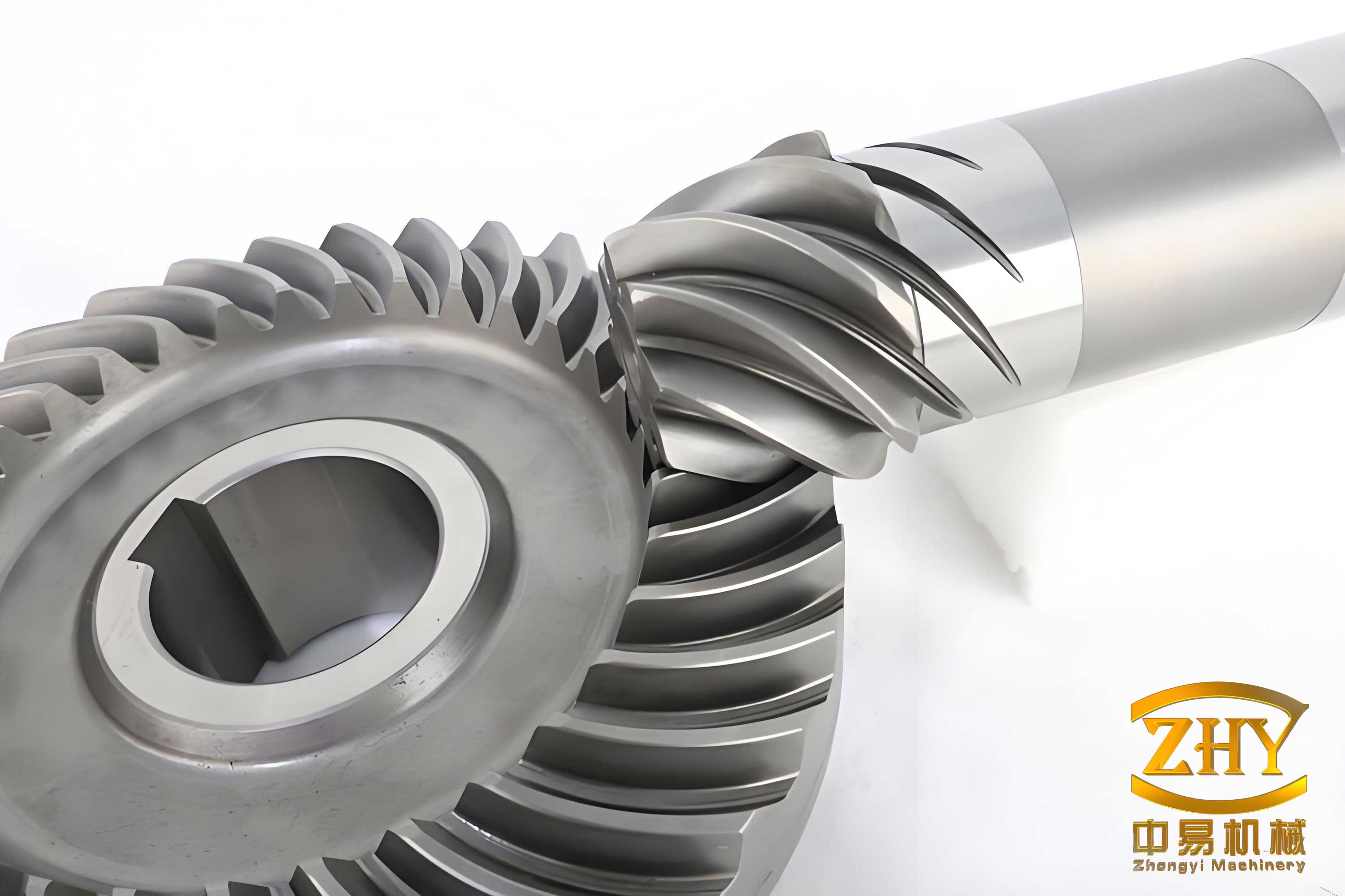
The reliable operation of mechanical drive systems is heavily dependent on the health of their critical components. Among these, the spiral bevel gearbox plays a pivotal role in transmitting power between non-parallel, intersecting shafts, commonly found in automotive differentials, helicopter transmissions, and heavy industrial machinery. Its failure can lead to catastrophic system downtime, costly repairs, and significant safety hazards. Therefore, developing accurate and robust fault diagnosis methods for spiral bevel gears is of paramount importance in modern predictive maintenance strategies.
Traditional fault diagnosis approaches for gearboxes have primarily relied on signal processing techniques like Empirical Mode Decomposition (EMD) and Variational Mode Decomposition (VMD) to extract meaningful features from vibration signals. While effective in controlled environments, these methods often struggle with the non-stationary, noisy signals characteristic of real-world industrial settings, especially for complex components like the spiral bevel gear. The advent of deep learning has ushered in a new era, with Convolutional Neural Networks (CNNs) and Recurrent Neural Networks (RNNs) like Long Short-Term Memory (LSTM) and Gated Recurrent Unit (GRU) networks showing remarkable success in learning discriminative features directly from raw or pre-processed data. However, significant challenges remain. Many existing deep learning models inadequately exploit the synergistic relationship between the spatial patterns in time-frequency representations and the long-term temporal dependencies in the raw vibration sequence. Furthermore, their performance and robustness can degrade substantially under strong background noise and varying operational conditions, which are unavoidable in practice.
To address these limitations, this paper proposes a novel intelligent fault diagnosis framework that synergistically combines a Receptive Field Attention-enhanced Residual Network (ResNet-RFA) and a Bidirectional Gated Recurrent Unit with Self-Attention (BiGRU-SATT). The core innovation lies in a dual-channel architecture designed to collaboratively mine spatiotemporal features. One channel processes a 2D time-frequency image generated via Short-Time Fourier Transform (STFT) using the ResNet-RFA module, which applies parameter-level attention to dynamically weight the convolutional kernel’s receptive field, enhancing focus on critical fault-related regions. The other channel processes the original 1D vibration signal using the BiGRU-SATT module, which captures bidirectional temporal context and employs self-attention to highlight the most relevant time steps for classification. The fused spatiotemporal features are then fed to a classifier. Experimental validation on a spiral bevel gearbox dataset demonstrates that this hybrid model achieves superior diagnostic accuracy and exhibits exceptional robustness against Gaussian-impulse mixed noise, outperforming several state-of-the-art and classical models.
Methodology
The proposed methodology encompasses three main stages: data preprocessing, dual-channel feature extraction, and fusion-based classification. The overall architecture is designed to fully leverage the complementary information present in different signal representations.
Data Preprocessing and Augmentation
Effective preprocessing is crucial for preparing the vibration data for deep learning models and mitigating the risk of overfitting, especially with limited labeled samples.
Overlapping Sampling: To artificially expand the training dataset and improve model generalization, overlapping sampling is applied to the raw vibration signals. A sliding window of length $w_X$ traverses the signal with a step size $L_s$, where $L_s < w_X$. This generates multiple, slightly shifted samples from a single continuous recording. The window length should be at least sufficient to cover one complete revolution of the gear to capture periodic fault signatures:
$$ w_X \geq \frac{60}{n} F_s $$
where $n$ is the rotational speed in RPM and $F_s$ is the sampling frequency in Hz. The total number of samples $N$ obtainable from a signal of length $L_t$ is given by:
$$ N \leq \frac{L_t – w_X}{L_s} + 1 $$
Time-Frequency Analysis via STFT: To transform the 1D temporal signal into a 2D representation that reveals joint time-frequency characteristics, Short-Time Fourier Transform (STFT) is employed. The continuous signal $x(t)$ is divided into short, possibly overlapping segments using a window function $w(t)$ (e.g., Hanning window). The STFT at time frame $m$ and frequency bin $k$ is computed as:
$$ \text{STFT}(m, k) = \sum_{t=0}^{L_w-1} x_m(t) \cdot e^{-j 2\pi k t / L_w} $$
where $x_m(t) = x(t) \cdot w(t – m L_s)$ is the windowed signal segment. The choice of window length $L_w$ involves a trade-off between time and frequency resolution and is often set as $L_w = \alpha \cdot \frac{F_s}{f_{\text{min}}}$, with $\alpha$ between 2 and 5 and $f_{\text{min}}$ being the lowest frequency of interest. The magnitude of the STFT is used to generate a time-frequency image (e.g., 256×256 pixels), which serves as the input to the spatial feature extraction channel.
Sequential Signal Preparation: Concurrently, the original 1D vibration samples (after overlapping sampling) are preserved and reshaped into appropriate sequential tensors to serve as input for the temporal modeling channel.
Spatial Feature Extraction with ResNet-RFA
This branch is responsible for learning discriminative spatial patterns from the STFT time-frequency images. It is built upon a Residual Network (ResNet) backbone, enhanced with a Receptive Field Attention (RFA) mechanism.
Residual Network Backbone: The ResNet structure mitigates the vanishing gradient problem in deep networks through skip connections. A basic residual block performs the operation:
$$ \mathbf{y} = \mathcal{F}(\mathbf{x}, \{W_i\}) + \mathbf{x} $$
where $\mathbf{x}$ is the input, $\mathbf{y}$ is the output, and $\mathcal{F}$ represents the residual mapping to be learned, typically consisting of two or three convolutional layers with batch normalization and ReLU activation.
Receptive Field Attention (RFA) Mechanism: Unlike standard spatial or channel attention, RFA operates at a finer, parameter-wise granularity. It generates a 4D attention tensor $A \in \mathbb{R}^{B \times C_{out} \times k \times k}$ that dynamically weights each parameter within the $k \times k$ convolutional kernel for every output channel. The process is as follows:
- Global Context Encoding: The input feature map $X$ undergoes global average pooling to produce a channel-wise descriptor vector $Z \in \mathbb{R}^{B \times C_{in}}$:
$$ Z_c = \frac{1}{H \times W} \sum_{i=1}^{H} \sum_{j=1}^{W} X_c(i, j) $$ - Attention Weight Generation: $Z$ is passed through a bottleneck structure with two fully connected layers and a non-linear activation (e.g., ReLU) to produce a raw weight tensor, which is then reshaped and normalized via a sigmoid function to obtain the final 4D attention tensor $A_{k \times k}$:
$$ A_{k \times k} = \sigma(\text{Reshape}(W_2 \delta(W_1 Z + b_1) + b_2)) $$
where $\sigma$ is the sigmoid function and $\delta$ is ReLU. - Multi-Scale Dynamic Convolution: Multiple depthwise separable convolutions with different kernel sizes (e.g., 3×3, 5×5, 7×7) are applied to the input. Their kernels are element-wise multiplied by the corresponding slices of $A$, creating dynamic kernels:
$$ F_{k \times k} = (K_{k \times k} \odot A_{k \times k}) \circledast X $$
where $\odot$ denotes element-wise multiplication and $\circledast$ denotes the depthwise separable convolution operation. - Weighted Fusion: The outputs from the different scaled branches are fused using adaptive weights $\{w_1, w_2, w_3\}$ learned from the global context vector $Z$:
$$ Y = w_1 \cdot F_{3\times3} + w_2 \cdot F_{5\times5} + w_3 \cdot F_{7\times7} $$
$$ \{w_1, w_2, w_3\} = \text{Softmax}(W_f Z + b_f) $$
The RFA module, integrated into the ResNet, allows the model to adaptively focus on the most relevant spatial regions and frequency bands within the time-frequency image, which is particularly beneficial for identifying localized fault patterns in spiral bevel gear signals.
Temporal Feature Extraction with BiGRU-SATT
This branch is designed to capture the long-range temporal dependencies and evolutionary patterns in the raw 1D vibration sequence, which are essential for diagnosing faults that manifest over time.
Bidirectional Gated Recurrent Unit (BiGRU): A GRU cell simplifies the LSTM by combining the forget and input gates into a single update gate $z_t$. Its operations at time step $t$ are defined as:
$$
\begin{aligned}
z_t &= \sigma(W_z x_t + U_z h_{t-1} + b_z) \\
r_t &= \sigma(W_r x_t + U_r h_{t-1} + b_r) \\
\tilde{h}_t &= \tanh(W_h x_t + U_h (r_t \odot h_{t-1}) + b_h) \\
h_t &= (1 – z_t) \odot h_{t-1} + z_t \odot \tilde{h}_t
\end{aligned}
$$
where $x_t$ is the input, $h_t$ is the hidden state, $z_t$ is the update gate, $r_t$ is the reset gate, and $\tilde{h}_t$ is the candidate activation. The BiGRU stacks a forward GRU that processes the sequence from past to future and a backward GRU that processes it from future to past. The final hidden state at each time step is the concatenation of both directions: $h_t = [\overrightarrow{h}_t; \overleftarrow{h}_t]$, providing contextual information from the entire sequence.
Self-Attention Mechanism (SATT): While BiGRU captures contextual information, it may not effectively weigh the importance of different time steps. A self-attention layer is appended to the sequence of BiGRU outputs $H = [h_1, h_2, …, h_T]$. It computes a weighted sum where the weights are determined by the compatibility of a query with a set of key-value pairs, all derived from $H$ itself:
$$
\begin{aligned}
Q = H W^Q, \quad K = H W^K, \quad V = H W^V \\
\text{Attention}(Q, K, V) = \text{Softmax}\left(\frac{QK^T}{\sqrt{d_k}}\right) V
\end{aligned}
$$
The output is a context vector that represents the entire sequence, with higher weights assigned to the most salient time steps for fault classification. This is especially useful for pinpointing the transient impact events caused by faults in a spiral bevel gear amidst continuous vibration.
Feature Fusion and Classification
The spatial feature vector $\mathbf{f}_{\text{spatial}}$ extracted by the ResNet-RFA branch (e.g., a 512-dimensional vector after global pooling) and the temporal feature vector $\mathbf{f}_{\text{temporal}}$ extracted by the BiGRU-SATT branch (e.g., a 256-dimensional context vector) are concatenated to form a joint spatiotemporal representation:
$$ \mathbf{f}_{\text{fused}} = [\mathbf{f}_{\text{spatial}}; \mathbf{f}_{\text{temporal}}] $$
This fused vector is then passed through a fully connected classification network, typically consisting of one or more linear layers with dropout and ReLU activation, culminating in a softmax layer that outputs the probability distribution over the different fault classes of the spiral bevel gearbox.
The architectural details of the proposed hybrid model are summarized in the following table.
| Branch | Layer/Module | Output Shape / Configuration | Purpose |
|---|---|---|---|
| Spatial (Image) | Input | (Batch, 3, 256, 256) | STFT time-frequency image (RGB) |
| Conv2D + BN + ReLU | (Batch, 64, 128, 128) | Initial feature extraction | |
| ResNet Blocks with RFA | Multiple blocks (e.g., 4 stages) | Hierarchical spatial feature learning with dynamic receptive field | |
| Global Average Pooling | (Batch, 512) | Generate spatial feature vector $\mathbf{f}_{\text{spatial}}$ | |
| Temporal (Signal) | Input | (Batch, Seq_Len, 1) | Raw 1D vibration sequence |
| BiGRU Layers | e.g., 2 layers, 128 hidden units each | Capture bidirectional long-term dependencies | |
| Self-Attention Layer | Heads=8, $d_k$=16 | Focus on critical time steps | |
| Context Vector | (Batch, 256) | Generate temporal feature vector $\mathbf{f}_{\text{temporal}}$ | |
| Fusion & Classification | Feature Concatenation | (Batch, 768) | Merge spatiotemporal features |
| FC + ReLU + Dropout | (Batch, 128) | Non-linear projection | |
| Softmax Classifier | (Batch, N_classes) | Output fault probabilities |
Experimental Setup and Dataset
The performance of the proposed model was evaluated using vibration data collected from a dedicated spiral bevel gearbox fault simulation test rig. The experimental setup is designed to replicate real operating conditions and induce common fault types.
Test Rig and Data Acquisition
The test rig comprises a drive motor, a torque sensor, the spiral bevel gearbox under test, a planetary gear reducer, a magnetic powder brake for loading, and a data acquisition system. Vibration signals were acquired using ICP accelerometers mounted on the housing of the gearbox. Data was collected under a constant motor speed of 1000 RPM and a sampling frequency of 5000 Hz.
Fault Conditions and Dataset Construction
Seven distinct health conditions were simulated to create a comprehensive dataset representative of common spiral bevel gear failures:
- Normal Condition (Healthy)
- Large Gear Missing Tooth
- Small Gear (Pinion) Missing Tooth
- Large Gear Root Crack
- Small Gear Root Crack
- Large Gear Surface Wear
- Small Gear Surface Wear
For each condition, 60 seconds of vibration data was recorded. The raw signal was then segmented using overlapping sampling with a window length $w_X$ = 1024 points (covering more than one revolution) and a step size $L_s$ = 128 points. This yielded 1120 samples per condition, resulting in a total of 7840 samples for the entire dataset. Each 1D sample was transformed into a 256×256 RGB time-frequency image via STFT for the spatial branch, while the original 1D sequence was kept for the temporal branch. The dataset was split into training and testing sets with an 80:20 ratio (6272 samples for training, 1568 for testing). The details of the constructed dataset are presented below.
| Fault Class | Label | Description | Samples (Total) | Samples (Train) | Samples (Test) |
|---|---|---|---|---|---|
| Normal | C0 | Healthy gearbox operation | 1120 | 896 | 224 |
| Large Gear Missing Tooth | C1 | Severe localized fault on the large gear | 1120 | 896 | 224 |
| Small Gear Missing Tooth | C2 | Severe localized fault on the pinion | 1120 | 896 | 224 |
| Large Gear Root Crack | C3 | Incipient crack at the tooth root of the large gear | 1120 | 896 | 224 |
| Small Gear Root Crack | C4 | Incipient crack at the tooth root of the pinion | 1120 | 896 | 224 |
| Large Gear Surface Wear | C5 | Distributed wear across the tooth surface of the large gear | 1120 | 896 | 224 |
| Small Gear Surface Wear | C6 | Distributed wear across the tooth surface of the pinion | 1120 | 896 | 224 |
| Total | 7840 | 6272 | 1568 | ||
Implementation Details and Evaluation Metrics
The model was implemented using PyTorch. The Adam optimizer was used with an initial learning rate of 0.001 and a weight decay of 1e-4. A learning rate scheduler was employed to reduce the rate upon plateau. The training was conducted for 30 epochs with a batch size of 32. Dropout with a rate of 0.5 was applied in the fully connected layers to prevent overfitting. The primary evaluation metric was classification accuracy on the independent test set. To assess robustness, Gaussian-impulse mixed noise was added to the original test signals at Signal-to-Noise Ratio (SNR) levels of 10 dB and 20 dB (with an impulse occurrence probability of 5%).
Results and Analysis
The experimental results are presented and analyzed from multiple perspectives to validate the effectiveness, robustness, and superiority of the proposed hybrid model.
Diagnostic Performance under Ideal Conditions
Under clean (noise-free) conditions, the proposed ResNet-RFA+BiGRU-SATT model demonstrated exceptional performance. The training and testing accuracy curves converged rapidly to 100%, and the corresponding loss values decreased smoothly to near zero. This indicates that the model not only learned the training data perfectly but also generalized flawlessly to unseen test samples, achieving a perfect classification score. The confusion matrix for the noise-free test set was purely diagonal, confirming that all 1568 test samples were correctly classified into their respective spiral bevel gear fault categories.
Robustness Analysis under Noisy Conditions
The true test of a practical diagnostic model is its performance in noisy environments. The model was evaluated by injecting Gaussian-impulse mixed noise into the test signals.
At 10 dB SNR: The model maintained remarkably high performance. The test accuracy stabilized near 100% after about 20 epochs, closely following the training accuracy. The loss curves also converged stably to a low value (around 0.2). The corresponding confusion matrix showed minimal off-diagonal elements, indicating only a handful of misclassifications. This demonstrates the model’s strong ability to suppress this level of noise and extract reliable fault features.
At 20 dB SNR: As expected, the stronger noise presented a greater challenge. The test accuracy curve exhibited noticeable fluctuations during training (e.g., a dip around epoch 10), and the convergence was slower compared to the 10 dB case. The test loss curve was more volatile. Nevertheless, the model eventually achieved a high accuracy level, and the confusion matrix, while showing more misclassifications than the 10 dB case, still indicated a dominant diagonal. This confirms the model’s inherent robustness, though performance degradation with increasing noise is observable.
The performance summary under different noise levels is quantified in the following table.
| Noise Condition (SNR) | Final Test Accuracy (%) | Final Test Loss | Convergence Stability | Key Observation |
|---|---|---|---|---|
| Noise-Free | 100.00 | ~0.001 | Excellent | Perfect classification, no misclassifications. |
| 10 dB Mixed Noise | >99.5 | ~0.2 | Very Good | Minimal performance drop, robust feature extraction. |
| 20 dB Mixed Noise | >98.0 | ~0.5 | Good (with fluctuations) | Increased misclassifications but maintains high overall accuracy. |
Model Stability and Statistical Significance
To ensure the results were not due to a fortunate random split, a comprehensive statistical analysis was conducted.
Repeated Trials: The experiment was repeated 30 times with random shuffling and splitting of the dataset. The proposed model achieved an average accuracy of 99.93% with a very small standard deviation of ±0.12%, proving its high stability and reproducibility.
Cross-Validation: A 5-fold cross-validation was performed. The model yielded consistent accuracy above 99.8% across all folds, with an average of 99.92% and a standard deviation of 0.0004. This confirms that the model’s performance is independent of the specific data partition and that overfitting is effectively controlled.
The average confusion matrix from the 30 repeated trials showed diagonal elements all exceeding 99.9%, with the maximum misclassification rate for any class being below 0.04%.
Comparative Study with Other Models
The performance of the proposed hybrid model was benchmarked against several prominent and classical models to highlight its advantages. The competitors included:
- Transformer: A pure attention-based model operating on sequence data.
- Mamba: A recent state-space model known for efficient long-sequence modeling.
- Support Vector Machine (SVM): A classical machine learning method with handcrafted features (time and frequency domain features were extracted for this baseline).
- Deep Belief Network (DBN): A classical deep learning model for unsupervised feature learning.
The comparison was conducted on the same spiral bevel gearbox dataset under clean conditions. The results, summarized in the table and figure below, clearly demonstrate the superiority of the proposed approach.
| Model | Type | Test Accuracy (%) | Remarks |
|---|---|---|---|
| Proposed (ResNet-RFA+BiGRU-SATT) | Hybrid Deep Learning | 100.00 | Superior accuracy and stability |
| Mamba | State-Space Model | 96.00 | Good performance, but lower than the hybrid model |
| SVM (with features) | Classical ML | 94.00 | Performance limited by quality of handcrafted features |
| Transformer | Attention-based | 91.00 | May require more data for optimal performance on this task |
| DBN | Deep Learning | 89.00 | Lower performance compared to modern architectures |
The proposed model outperformed all others, achieving perfect accuracy. The Mamba model performed respectably at 96%, showcasing the potential of new sequence modeling paradigms. The classical SVM, while competitive, was limited by its dependency on manual feature engineering. The Transformer and DBN models showed relatively lower performance on this specific gearbox fault diagnosis task. This comparative study validates the effectiveness of the dual-channel design for spiral bevel gear fault diagnosis, which successfully leverages both spatial and temporal information where other models may focus predominantly on one aspect.
Complexity and Real-Time Feasibility Analysis
For industrial deployment, computational efficiency is crucial. The proposed model’s complexity stems from its dual branches. The ResNet-RFA branch’s cost is related to the image dimensions and channel operations, while the BiGRU-SATT branch’s cost depends on sequence length and hidden dimensions. Profiling on an NVIDIA RTX 3080 GPU showed a single inference time of approximately 12.3 milliseconds, a parameter count of 18.7 million, and a memory footprint of around 320 MB. This demonstrates that the model can perform real-time diagnosis on suitable industrial computing hardware or edge devices with moderate resources. For deployment on very resource-constrained platforms, techniques like input down-sampling, model pruning, or quantization could be applied to further reduce the computational load.
Conclusion
This paper presented a novel intelligent fault diagnosis framework for spiral bevel gearboxes based on a hybrid deep learning model integrating ResNet-RFA and BiGRU-SATT. The core contribution is a dual-channel architecture that synergistically extracts and combines discriminative spatial features from time-frequency images and deep temporal dependencies from raw vibration sequences. The ResNet-RFA module introduces parameter-level receptive field attention to dynamically focus on critical fault patterns in the time-frequency domain. The BiGRU-SATT module effectively models long-range bidirectional context and uses self-attention to highlight the most relevant temporal events.
Extensive experiments on a dedicated spiral bevel gearbox dataset demonstrated that the proposed model achieves perfect (100%) classification accuracy under ideal conditions and maintains high accuracy and robustness under significant Gaussian-impulse mixed noise interference (10 dB and 20 dB SNR). Statistical analyses confirmed the model’s stability and generalizability. A comprehensive comparative study showed that the proposed model significantly outperforms other advanced and classical models, including Transformer, Mamba, SVM, and DBN.
The proposed method effectively addresses the challenges of spatiotemporal feature co-learning and noise robustness in complex gearbox fault diagnosis. It provides a powerful and reliable tool for the condition monitoring and predictive maintenance of spiral bevel gear transmission systems, with promising potential for real-world industrial application. Future work will focus on extending the model’s capability to handle variable speed conditions, exploring knowledge distillation for edge deployment, and testing its performance on broader types of rotating machinery faults.