
The pursuit of superior performance in gear transmissions, particularly for spiral bevel and hypoid gears, has consistently focused on achieving higher load capacity and lower noise levels. The real tooth flank geometry, however, invariably deviates from the theoretically designed or precisely defined standard due to a multitude of factors including heat treatment distortion, variations in cutting forces, and other unpredictable elements in the manufacturing process. These deviations lead to problematic edge contacts, concentrated stress, premature failure, and increased transmission noise. Therefore, it is critically important to perform corrective adjustments to the manufacturing parameters—a process known as machine settings modification or compensation—prior to the actual cutting process, to proactively counteract these potential errors.
Over the past decades, various gear generation systems, predominantly from Gleason and Klingelnberg, have been developed for specific machine types. While effective, this diversity often results in a proliferation of adjustment processes that can be complex, inefficient, and may not achieve the highest possible precision. In recent years, closed-loop modification theories have gained prominence. These methodologies are fundamentally based on error sensitivity analysis and the correction of the tooth flank’s ease-off topography. Ease-off, defined as the normal deviation between two mating flanks or between a real and theoretical flank, serves as a comprehensive metric for tooth surface error. By strategically modifying the machine settings to minimize the ease-off, a high-precision, high-performance tooth surface conducive to favorable contact patterns and low noise can be manufactured.
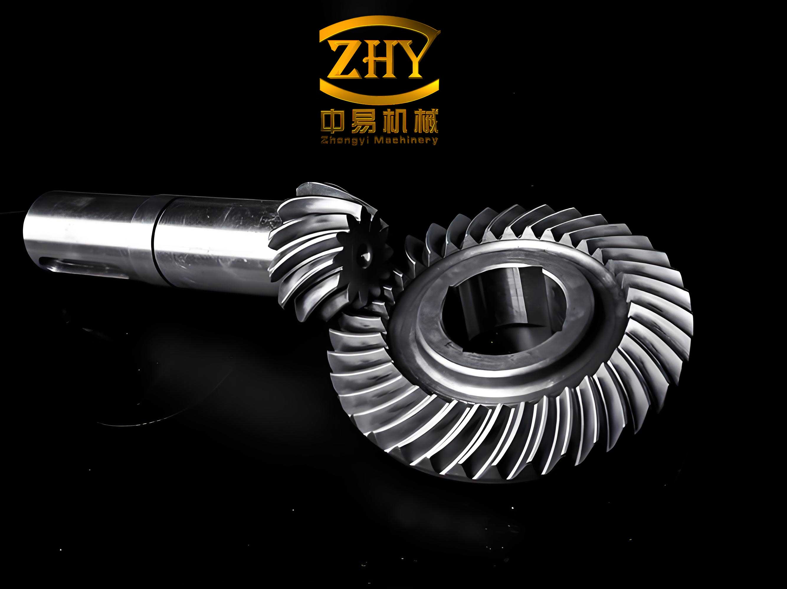
The concept of Universal Motion Concept (UMC) and its subsequent evolution into the Universal Generation Model (UGM) have provided a powerful framework for unifying these diverse machining methods. The UGM employs a set of universal machine tool settings, which are parameters describing the relative positions and motions between the cutter and the gear blank. The key innovation enabling high-precision correction is the expression of these settings not as constants, but as higher-order polynomial functions of the cradle rotation angle. This parameterization introduces sufficient degrees of freedom to generate and subsequently correct complex flank topography with high accuracy. This article delves into a comprehensive methodology for the higher-order anti-correction modification of universal machine settings, targeting the precise minimization of the ease-off topography for spiral bevel gears.
Theoretical Foundation: Universal Generation Model and Higher-Order Settings
Manufacturing methods for spiral bevel gears can generally be categorized into two main types: the single-indexing face milling method (typical of Gleason systems) and the continuous indexing face hobbing method (typical of Klingelnberg systems). The Universal Generation Model (UGM) elegantly unifies these and other methods by describing the process using a generalized set of kinematic parameters. As illustrated in the referenced model, these parameters define the spatial relationship between the cutter axis and the gear blank axis.
In conventional machining, these settings are often constants. For high-order modification, however, they are defined as polynomial functions of the cradle angle, $$q$$ (or sometimes denoted as $$\phi_c$$). This allows the machine to execute complex, non-linear motions during the generation process, which is essential for creating and correcting sophisticated flank modifications like tip and root relief, bias, and crowning. The universal machine settings can be expressed as:
| Machine Setting | Symbol | Higher-Order Polynomial Expression |
|---|---|---|
| Ratio of Roll | $$R_a$$ | $$R_a(q) = R_{a0} + R_{a1} \Delta q + R_{a2} \Delta q^2 + … + R_{an} \Delta q^n$$ |
| Cutter Tilt Angle | $$\sigma$$ | $$\sigma(q) = \sigma_0 + \sigma_1 \Delta q + \sigma_2 \Delta q^2 + … + \sigma_n \Delta q^n$$ |
| Cutter Swivel Angle | $$\zeta$$ | $$\zeta(q) = \zeta_0 + \zeta_1 \Delta q + \zeta_2 \Delta q^2 + … + \zeta_n \Delta q^n$$ |
| Radial Distance | $$S_r$$ | $$S_r(q) = S_{r0} + S_{r1} \Delta q + S_{r2} \Delta q^2 + … + S_{rn} \Delta q^n$$ |
| Workpiece Offset | $$E_m$$ | $$E_m(q) = E_{m0} + E_{m1} \Delta q + E_{m2} \Delta q^2 + … + E_{mn} \Delta q^n$$ |
| Sliding Base | $$X_b$$ | $$X_b(q) = X_{b0} + X_{b1} \Delta q + X_{b2} \Delta q^2 + … + X_{bn} \Delta q^n$$ |
| Blank Tilt Angle | $$\gamma_m$$ | $$\gamma_m(q) = \gamma_{m0} + \gamma_{m1} \Delta q + \gamma_{m2} \Delta q^2 + … + \gamma_{mn} \Delta q^n$$ |
Where $$\Delta q = q – q_0$$, and $$q_0$$ is the initial cradle angle. Similar expressions apply to other settings like machine root angle, axial distance, etc. The order $$n$$ of the polynomial determines the complexity of the motion that can be modeled.
The mathematical model of the generated spiral bevel gear tooth surface is derived through a series of coordinate transformations from the cutter coordinate system to the workpiece coordinate system. The surface can be represented parametrically. Let $$\mathbf{r}_c(u, \theta)$$ be the cutter surface vector, defined by its surface parameters $$u$$ and $$\theta$$. The transformation through the machine kinematics involves matrices that account for the cutter head geometry, the machine settings (which are now functions of $$q$$), and the rolling motion between the cradle and the workpiece. The generated gear tooth surface $$\mathbf{R}_g$$ and its unit normal vector $$\mathbf{n}_g$$ are functions of the cutter parameters, the motion parameter (cradle angle $$q$$, which is linked to the workpiece rotation $$\phi$$ via the ratio of roll $$R_a(q)$$), and the complete set of machine setting functions, denoted collectively as the vector $$\boldsymbol{\xi}(q)$$:
$$
\mathbf{R}_g = \mathbf{R}_g(u, \theta, q; \boldsymbol{\xi}(q)), \quad \mathbf{n}_g = \mathbf{n}_g(u, \theta, q; \boldsymbol{\xi}(q))
$$
The fundamental equation of meshing, $$\mathbf{n} \cdot \mathbf{v}^{(12)} = 0$$, where $$\mathbf{v}^{(12)}$$ is the relative velocity between the cutter and the blank, provides an additional constraint that allows the elimination of one parameter (typically $$q$$), resulting in the final tooth surface expressed as a function of two independent parameters: $$\mathbf{R}_g = \mathbf{R}_g(u, \theta; \boldsymbol{\xi})$$ and $$\mathbf{n}_g = \mathbf{n}_g(u, \theta; \boldsymbol{\xi})$$. The vector $$\boldsymbol{\xi}$$ now encapsulates all the polynomial coefficients from every machine setting function, making it a high-dimensional vector: $$\boldsymbol{\xi} = [R_{a0}, R_{a1}, …, \sigma_0, \sigma_1, …, S_{r0}, …]^T$$.
Methodology for Higher-Order Machine Settings Anti-Correction
1. Modeling the Real Flank with Errors
In practice, the actual manufactured flank of a spiral bevel gear deviates from the theoretical target surface. This real flank can be considered as being generated by a perturbed set of machine settings $$\boldsymbol{\xi}’ = \boldsymbol{\xi} + \Delta\boldsymbol{\xi}$$, where $$\Delta\boldsymbol{\xi}$$ represents the unknown error increments in all polynomial coefficients arising from machine inaccuracies, tool wear, deflection, etc. The real surface measured on a Coordinate Measuring Machine (CMM) is denoted as $$\mathbf{R}_m(u_i, \theta_j)$$ at discrete grid points indexed by $$i$$ (along the profile direction) and $$j$$ (along the lengthwise direction).
The ease-off topography, $$\delta(u, \theta)$$, is then defined as the normal distance from a point on the measured real surface to the theoretical designed surface. For a discrete measurement point corresponding to a theoretical point $$\mathbf{R}_g(u_i, \theta_j)$$ with normal $$\mathbf{n}_g(u_i, \theta_j)$$, the ease-off value is calculated as:
$$
\delta_{ij} = \left[ \mathbf{R}_m(u_i, \theta_j) – \mathbf{R}_g(u_i, \theta_j; \boldsymbol{\xi}) \right] \cdot \mathbf{n}_g(u_i, \theta_j)
$$
This set of $$\delta_{ij}$$ values forms a discrete error map or ease-off surface that quantitatively represents the manufacturing error of the spiral bevel gear flank.
2. Error Sensitivity Analysis and Formulation of the Correction Problem
A small change in the machine setting coefficients $$\Delta\boldsymbol{\xi}$$ will induce a corresponding change in the theoretical tooth surface point location. A first-order approximation of this change, projected onto the surface normal, gives the resulting change in ease-off. This relationship forms the basis of sensitivity analysis.
The sensitivity of the ease-off at point $$(i,j)$$ to a change in the $$k$$-th machine setting coefficient $$\xi_k$$ is given by the partial derivative:
$$
S_{ij,k} = \frac{\partial \delta_{ij}}{\partial \xi_k} \approx \frac{\partial \mathbf{R}_g(u_i, \theta_j; \boldsymbol{\xi})}{\partial \xi_k} \cdot \mathbf{n}_g(u_i, \theta_j)
$$
This sensitivity coefficient $$S_{ij,k}$$ can be computed efficiently using the tooth surface model and differential geometry. For all measurement points and all adjustable coefficients, this relationship can be assembled into a linearized matrix equation:
$$
\{\Delta \boldsymbol{\delta}\} = [\mathbf{S}] \{\Delta \boldsymbol{\xi}\}
$$
Here, $$\{\Delta \boldsymbol{\delta}\}$$ is a column vector containing all $$M$$ measured ease-off values $$\delta_{ij}$$ (flattened from the grid). $$\{\Delta \boldsymbol{\xi}\}$$ is the column vector of $$N$$ unknown correction increments for the machine setting coefficients. $$[\mathbf{S}]$$ is the $$M \times N$$ sensitivity matrix (or Jacobian matrix), where each element is $$S_{ij,k}$$.
The goal of the anti-correction modification is to find the optimal set of corrections $$\Delta \boldsymbol{\xi}$$ such that the new ease-off, after applying the corrections, is minimized. This is formulated as a nonlinear least-squares problem:
$$
\min_{\Delta \boldsymbol{\xi}} f(\Delta \boldsymbol{\xi}) = \frac{1}{2} \| \boldsymbol{\delta}_{meas} – \mathbf{S}(\boldsymbol{\xi}) \Delta \boldsymbol{\xi} \|^2
$$
Where $$\boldsymbol{\delta}_{meas}$$ is the vector of measured ease-off values from the initial (erroneous) spiral bevel gear. Due to the inherent nonlinearity of the gear generation process (the sensitivity matrix $$\mathbf{S}$$ itself is a function of the current settings $$\boldsymbol{\xi}$$), this problem is strongly nonlinear and often ill-conditioned, requiring robust numerical algorithms for solution.
3. Solution via Improved Levenberg-Marquardt Algorithm with Trust Region
To solve this nonlinear minimization problem robustly, an improved Levenberg-Marquardt (L-M) algorithm incorporating a trust-region strategy is employed. The standard L-M algorithm iteratively updates the solution by solving:
$$
(\mathbf{J}^T \mathbf{J} + \mu \mathbf{I}) \mathbf{h}_{lm} = -\mathbf{J}^T \mathbf{f}
$$
where $$\mathbf{J}$$ is the Jacobian matrix (our sensitivity matrix $$\mathbf{S}$$), $$\mathbf{f}$$ is the residual vector ($$\boldsymbol{\delta}_{meas} – \mathbf{S} \Delta \boldsymbol{\xi}_{current}$$), $$\mu$$ is a damping parameter, $$\mathbf{I}$$ is the identity matrix, and $$\mathbf{h}_{lm}$$ is the computed step ($$\Delta \boldsymbol{\xi}_{new}$$).
The trust-region strategy improves stability by constraining the step size. At each iteration $$k$$, the algorithm approximately solves a subproblem within a trust region of radius $$\Delta_k$$:
$$
\min_{\mathbf{h}} f_k(\mathbf{h}) = f(\boldsymbol{\xi}_k) + \mathbf{g}_k^T \mathbf{h} + \frac{1}{2} \mathbf{h}^T \mathbf{G}_k \mathbf{h}, \quad \text{subject to} \quad \|\mathbf{h}\| \leq \Delta_k
$$
where $$\mathbf{g}_k = \mathbf{J}_k^T \mathbf{f}_k$$ is the gradient and $$\mathbf{G}_k \approx \mathbf{J}_k^T \mathbf{J}_k$$ is an approximation of the Hessian. The quality of the step is evaluated by the ratio $$\rho_k$$ of the actual reduction in the objective function to the predicted reduction:
$$
\rho_k = \frac{f(\boldsymbol{\xi}_k) – f(\boldsymbol{\xi}_k + \mathbf{h}_k)}{f_k(\mathbf{0}) – f_k(\mathbf{h}_k)}
$$
The trust region radius $$\Delta_k$$ and the damping parameter $$\mu_k$$ are adaptively adjusted based on $$\rho_k$$:
$$
\text{If } \rho_k < 0.25: \quad \Delta_{k+1} = 0.25 \Delta_k, \quad \mu_{k+1} = \Delta_k \cdot \mu_k
$$
$$
\text{If } \rho_k > 0.75 \text{ and } \|\mathbf{h}_k\| = \Delta_k: \quad \Delta_{k+1} = \min(2\Delta_k, \Delta_{max}), \quad \mu_{k+1} = \mu_k / \Delta_k
$$
$$
\text{Otherwise}: \quad \Delta_{k+1} = \Delta_k, \quad \mu_{k+1} = \mu_k
$$
This iterative process continues until convergence criteria are met, such as a sufficiently small gradient norm $$\|\mathbf{g}_k\|$$, a small change in parameters $$\|\mathbf{h}_k\|$$, or a minimal residual norm $$\|\mathbf{f}_k\|$$. The final output is the vector of optimal correction increments $$\Delta \boldsymbol{\xi}_{opt}$$ to be applied to the machine settings’ polynomial coefficients.
4. Procedure for Higher-Order Ease-Off Correction
The complete higher-order modification methodology for spiral bevel gears involves the following steps:
- Initial Manufacturing and Measurement: A spiral bevel gear pinion or gear is cut using a set of nominal machine settings (which may be constant or low-order). The real tooth flanks are precisely measured on a CMM to obtain point cloud data $$\mathbf{R}_m$$.
- Ease-Off Calculation: The measured points are aligned with the theoretical flank model, and the ease-off topography $$\delta_{meas}(u, \theta)$$ is computed at a defined grid of points.
- Sensitivity Matrix Computation: Based on the current (nominal) machine settings $$\boldsymbol{\xi}$$, the sensitivity matrix $$\mathbf{S}$$ is calculated for all grid points with respect to a selected subset of the most influential higher-order coefficients. This selection is crucial for problem conditioning; typically, 3-5 key parameters (like the constant and linear terms of ratio of roll, cradle angle, and radial distance) are chosen based on preliminary sensitivity screening.
- Iterative Solution for Corrections: The improved L-M algorithm with trust region is used to solve the nonlinear least-squares problem, yielding the optimal correction increments $$\Delta \boldsymbol{\xi}_{opt}$$.
- High-Order Ease-Off Representation (Optional Refinement): The residual ease-off after the primary correction can be further characterized. It can be approximated by a bi-variate polynomial function over the flank grid:
$$
\delta^*(x, y) = c_0 + c_1 x + c_2 y + c_3 x^2 + c_4 x y + c_5 y^2 + c_6 x^3 + …
$$Where $$x$$ and $$y$$ represent coordinates on the tooth flank (e.g., along profile and lengthwise). The coefficients $$c_i$$ have geometric interpretations: $$c_1, c_2$$ relate to flank slope (spiral angle and pressure angle errors); $$c_3, c_4, c_5$$ relate to second-order errors like profile curvature, twist, and lengthwise curvature. This explicit form can guide further selective higher-order term adjustments in the machine settings to target specific error components.
- Verification: The corrected machine settings $$\boldsymbol{\xi}_{new} = \boldsymbol{\xi} + \Delta \boldsymbol{\xi}_{opt}$$ are used to simulate the generation of a new tooth flank. The ease-off between this simulated corrected flank and the ideal target flank is computed. This virtual verification confirms the effectiveness of the modification before actual re-machining.
Numerical Example and Results
To validate the proposed methodology, a case study was performed on a spiral bevel gear pinion. The initial gear was manufactured, and its flanks were measured. A first-order (linear) correction was first applied to a subset of key machine settings. The sensitivity analysis identified parameters like the constant term of the basic cradle angle ($$q_0$$), the constant term of the ratio of roll ($$R_{a0}$$), and the constant term of the eccentric angle ($$\beta_0$$) as highly influential. The following table summarizes the initial settings and the first-order corrections obtained for the convex and concave flanks.
| Machine Setting Coefficient | Nominal Value | Correction for Concave Flank ($$\Delta \xi$$) | Correction for Convex Flank ($$\Delta \xi$$) |
|---|---|---|---|
| $$q_0$$ (deg) | 112.2 | -0.148 | -5.848 |
| $$R_{a0}$$ | 6.3392 | -0.01004 | -0.00017 |
| $$\beta_0$$ (deg) | 81.9 | 0.714 | 4.382 |
Applying these corrections and simulating the new flank led to a significant reduction in ease-off. The maximum absolute ease-off values were reduced to the micron level. For the concave flank, the ease-off range was approximately $$[-0.67, 0.60] \, \mu m$$. For the convex flank, the range was approximately $$[-0.16, 0.13] \, \mu m$$.
To achieve even higher precision, a higher-order correction was implemented. By allowing the basic cradle angle $$q$$ to vary as a 5th-order polynomial, its coefficients were optimized. The table below shows the optimized higher-order coefficients for $$q$$ and the corresponding coefficients of the polynomial fit to the residual ease-off surface after this high-order correction.
| Coefficient Order for $$q(q)$$ | Optimized Value (Concave) | Optimized Value (Convex) | Ease-off Fit Coef. $$c_i$$ (Concave) [$$\mu m$$] | Ease-off Fit Coef. $$c_i$$ (Convex) [$$\mu m$$] |
|---|---|---|---|---|
| Constant ($$q_0$$) | 112.200 | 104.933 | 0 (ref.) | 0 (ref.) |
| Linear ($$q_1$$) | 0.06436 | 0.08972 | 1.211e-3 | 7.028e-3 |
| Quadratic ($$q_2$$) | -2.71e-3 | 1.681e-4 | -6.314e-4 | 4.102e-5 |
| Cubic ($$q_3$$) | 1.118e-4 | -7.719e-3 | 6.112e-7 | 8.2e-7 |
| 5th-order ($$q_5$$) | 9.01e-7 | -4.01e-6 | -3.319e-8 | -2.78e-9 |
The result of this high-order modification was a dramatic further reduction in the ease-off topography. The residual errors were flattened and minimized across the entire active flank area of the spiral bevel gear, confirming the efficacy of using higher-order universal machine settings for ultra-precise flank correction.
Conclusion
This article has presented a comprehensive and robust methodology for the higher-order anti-correction modification of spiral bevel gears, centered on the minimization of the ease-off topography using universal machine tool settings. The core of the method lies in the parameterization of machine settings as polynomial functions of the motion parameter, providing the necessary degrees of freedom for high-precision flank error correction. The integration of error sensitivity analysis with an improved Levenberg-Marquardt algorithm featuring a trust-region strategy ensures stable and accurate solutions to the strongly nonlinear inverse problem of finding optimal machine setting adjustments.
The proposed flow, encompassing real flank measurement, sensitivity-based optimal parameter selection, iterative correction solving, and optional high-order ease-off characterization, forms a closed-loop correction system. Numerical examples demonstrate that this approach can effectively reduce flank errors to the micrometer level and below. This methodology provides a unified theoretical foundation for the high-performance design and manufacturing of various types of spiral bevel and hypoid gears across different generation systems, significantly enhancing the potential for achieving optimal contact patterns, high strength, and low noise in final gear drives.