
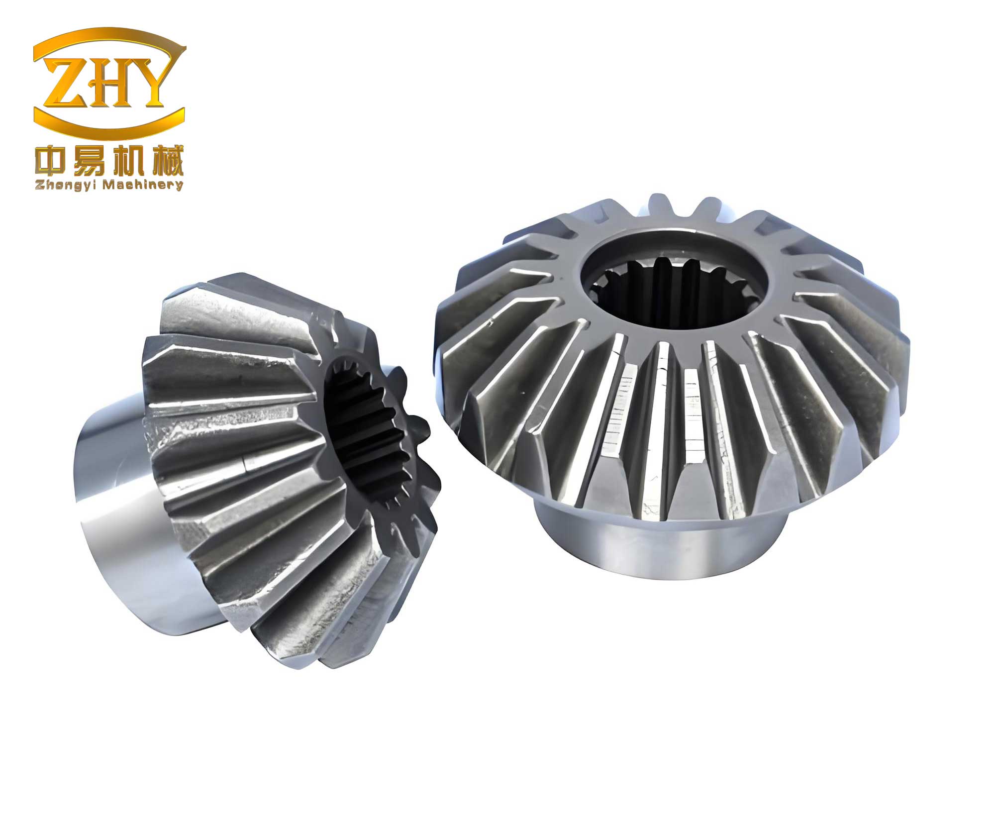
In the manufacturing of bevel gears, which are critical components in various mechanical transmission systems such as automotive differentials and aerospace applications, the precision of gear tooth profiles directly impacts performance, noise, and longevity. Bevel gear milling machines are specialized equipment used to produce these gears, and the spindle cutter disc assembly is a key subsystem responsible for holding and rotating the cutting tools. The assembly accuracy of this component—comprising the spindle, cutter disc, and housing—directly influences the final gear quality. However, part machining errors accumulate during assembly, leading to deviations that can compromise gear geometry. Therefore, analyzing geometric feature errors, establishing assembly error propagation models, and optimizing tolerances are essential for ensuring high-precision manufacturing of bevel gears. This article delves into these aspects, presenting a comprehensive methodology from error modeling to tolerance optimization, specifically tailored for bevel gear milling machine applications.
The foundation of assembly quality lies in part machining accuracy. To address this, we first focus on geometric feature error modeling. Traditional tolerance representation methods often lack completeness for complex surfaces like conical faces common in bevel gear tooling. Here, we employ the Small Displacement Torsor (SDT) method, a vectorial approach representing infinitesimal rigid body displacements with six components: three rotations (α, β, δ) and three translations (u, v, w). This method is well-suited for modeling deviations of geometric features due to tolerances. For instance, consider a conical surface, frequently encountered in spindle tapers for tool holding. The tolerance is often specified using the basic cone method, controlling both diameter and conical angle errors. Let the cone have a base radius R, height h, and taper 1:n. The total tolerance zone T is defined by upper and lower deviations, $T_U$ and $T_L$, such that $T = T_U + T_L$. The cone generatrix, represented as a line, can deviate within this zone. Its SDT parameters, considering relevant degrees of freedom, are (α, β, 0, u, v, 0). By deriving the boundary equations of the tolerance zone and analyzing extreme rotations, we establish inequalities for the variation ranges of α and v. For a conical surface, after simplification assuming small angles (sin α ≈ α, cos α ≈ 1), the inequalities are:
$$ -\frac{Th}{\sqrt{h^2 + (h/n + T)^2} \sqrt{h^2 + (h/n – T)^2}} \leq \alpha \leq \frac{Th}{\sqrt{h^2 + (h/n + T)^2} \sqrt{h^2 + (h/n – T)^2}} $$
$$ -T \leq v \leq T $$
with additional constraints ensuring the generatrix stays within the radial limits. Similar SDT-based models are developed for other features crucial in the assembly, such as planes, cylindrical surfaces, and axes. The table below summarizes the SDT expressions and variation inequalities for these features, which are foundational for subsequent analysis.
| Geometric Feature | SDT Expression (relevant components) | Variation Inequalities & Constraints |
|---|---|---|
| Plane (with size & perpendicularity tolerances) | (α, β, 0, 0, 0, w) | $-T_L/2c \leq \alpha \leq T_U/2c$, $-T_L/2b \leq β \leq T_U/2b$, $-T_O \leq w \leq T_O$; Constraints involve combined effects of α, β, w and size. |
| Cylindrical Surface (with size & cylindricity tolerances) | (α, β, 0, u, v, 0) | $-\frac{T_L + t}{h} \leq \alpha \leq \frac{T_U + t}{h}$, $-(T_L – t) \leq v \leq (T_U – t)$; Constraint: $v + \alpha z$ within radial limits. |
| Axis (with straightness & position tolerances) | (α, β, 0, u, v, 0) | $-\frac{T_P + T_F}{h} \leq \alpha \leq \frac{T_P + T_F}{h}$, $-T_P \leq v \leq T_P$; Constraint: $|\alpha z + v| \leq T_P$. |
However, these inequalities define the maximum possible ranges. The actual statistical distribution of errors is needed for robust analysis. We employ the Monte Carlo Simulation (MCS) method to estimate the actual variation bandwidth of SDT parameters. Assuming error components follow a normal distribution truncated within the tolerance zone (with mean at the range center and standard deviation derived from a ±3σ span), we generate a large number of random samples (e.g., 10,000) for parameters like α and v. Samples are accepted only if they satisfy the constraint inequalities. For the conical surface example, we check if the generated (α, v) pair keeps the generatz within $[R – T_L – h/(2n), R + T_U – h/(2n)]$. The accepted samples are then fitted to a distribution (verified by chi-square test), and its mean ($\hat{\mu}$) and standard deviation ($\hat{\sigma}$) are estimated via maximum likelihood. The actual bandwidth $D_i$ for parameter i (e.g., α) is then $D_i = 6\hat{\sigma}_i / G$, where G is a relative distribution coefficient (G=1 for normal). This process is repeated for all SDT parameters of all features.
To establish a continuous relationship between these bandwidths and the tolerance values, we use the Response Surface Method (RSM). For each geometric feature, we vary its associated tolerances (e.g., size tolerance T, cylindricity t) within their specified design ranges. At each discrete combination (experimental point), we compute the bandwidths via MCS. Then, we fit a second-order polynomial without cross-terms to model each bandwidth as a function of the tolerances. For a conical surface error parameter $D_j$ (j representing α or v), the model is:
$$ D_j = c_0 + c_1 T + c_2 n + c_3 T^2 + c_4 T n + c_5 n^2 $$
where T is the size tolerance and n is the taper parameter. Coefficients $c_0$ to $c_5$ are determined using least squares regression. The model’s accuracy is assessed by the coefficient of determination $R^2$, ensuring a close fit. This approach yields explicit functions $D_{α}(T, n)$ and $D_{v}(T, n)$, which are crucial for efficient error propagation analysis and optimization. Similar response surface models are created for plane and cylindrical feature error bandwidths.
With geometric feature errors characterized, we move to assembly error propagation. The spindle cutter disc assembly involves multiple mating interfaces: cylindrical fits (e.g., bearing seats), conical fits (spindle taper to cutter disc), and planar fits (face contacts). Each mating interface acts as an error source and transmitter. We model the error at a mating interface as the relative displacement between the ideal and actual features of the two parts in contact. The process is conceptualized as: ideal feature of part A → actual feature of part A → actual feature of part B → ideal feature of part B. The cumulative error across this chain is computed by combining SDTs or, equivalently, using homogeneous transformation matrices. For a conical mating interface (common in tool holders for bevel gear cutters), assume a clearance fit. The error SDT for the conical pair, $[α_{34}, β_{34}, 0, u_{34}, v_{34}, 0]$, is derived as the sum of three contributions: the machining error of the male cone (spindle), the machining error of the female cone (cutter disc), and the error due to clearance. For an interference fit, the clearance contribution is zero. The corresponding transformation matrix $M_{34}$ representing this error is:
$$ M_{34} = \begin{bmatrix} 1 & -β_{34} & 0 & u_{34} \\ β_{34} & 1 & 0 & v_{34} \\ 0 & 0 & 1 & 0 \\ 0 & 0 & 0 & 1 \end{bmatrix} $$
Similarly, for cylindrical and planar mating surfaces, error matrices are derived. The table below summarizes the error models for key mating types.
| Mating Type | Error Transformation Matrix M | Key SDT Components |
|---|---|---|
| Cylindrical Fit (clearance) | $\begin{bmatrix} 1 & -β & 0 & u \\ β & 1 & 0 & v \\ 0 & 0 & 1 & 0 \\ 0 & 0 & 0 & 1 \end{bmatrix}$ | u, v depend on part errors and clearance. |
| Planar Fit (non-fixed) | $\begin{bmatrix} 1 & -β & 0 & 0 \\ β & 1 & 0 & 0 \\ 0 & 0 & 1 & w \\ 0 & 0 & 0 & 1 \end{bmatrix}$ | w depends on flatness/parallelism errors. |
Interfaces can be connected in series or parallel. In series, error propagates along a single path. In parallel, multiple interfaces share the connection between two parts, complicating error transmission. The error transmission properties of a mating interface are classified into strongly constrained (SC), weakly constrained (WC), and unconstrained (UC) degrees of freedom (DOF). Strong constraints are directions where error causes interference; weak constraints allow small play; unconstrained DOFs are free. For example, a cylindrical clearance fit strongly constrains radial translations (u,v), weakly constrains rotations (α,β), and leaves axial translation (w) and rotation (δ) unconstrained. For parallel mating, like a conical fit and a planar face contact together mounting the cutter disc to the spindle, we must determine the effective constraints. The assembly sequence matters; the first-engaged interface (e.g., the cone) is the primary constraint. The actual constraint sets for parallel interfaces are derived by considering potential interferences. If a secondary interface’s strong constraint conflicts with the primary’s strong or weak constraint, adjustments in part tolerances or assembly alignment are needed to avoid jamming. The actual error transmission properties $A_{Rpg}$ for a parallel group are the union of the actual strong constraint sets $P_{RS}$ and weak constraint sets $P_{RW}$ of all interfaces, computed after resolving conflicts based on assembly order.
Building on this, we establish the complete error propagation model for the spindle cutter disc assembly. The assembly chain starts from the housing reference, goes through bearing fits (cylindrical), the spindle, the conical taper, the planar face contact, and ends at the cutter disc’s working plane. The total error at the cutter disc, represented as a displacement vector [u, v, w] at a point of interest, is computed by multiplying the sequence of transformation matrices: ideal housing feature → actual housing feature → … → ideal cutter disc feature. Each matrix is either an error matrix for a mating interface or a nominal coordinate transformation between feature locations. The final expression combines all error contributions from part machining and fits. Using the response surface models for individual feature error bandwidths, we can compute the statistical characteristics of the final assembly error [u, v, w] via Monte Carlo simulation of the entire chain.
To ensure the assembly meets precision requirements despite variations, we incorporate reliability analysis. Let the critical assembly precision requirement be that the resultant error at the cutter disc, say the radial runout $D_c = \sqrt{u^2 + v^2}$, is less than a threshold $r$ (e.g., 0.035 mm). The limit state function is $g(T) = r – D_c(T)$, where T is the vector of all tolerances. The system is reliable if $g(T) > 0$. The reliability $R(T)$ is the probability that this holds. We estimate $R(T)$ using Monte Carlo simulation over the tolerance distributions. For a given set of tolerances, we sample the SDT parameters based on their distributions, propagate through the error model, compute $D_c$, and count the fraction of samples where $D_c < r$. This fraction is the estimated reliability.
The goal of tolerance optimization is to minimize manufacturing cost while satisfying reliability and design rules. The cost of achieving a tolerance is inversely related to its magnitude; tighter tolerances cost more. We use established tolerance-cost models for different feature types. For example, for planar features with size and geometric tolerances, a combined cost model might be: $C(T) = e^{-15.8903T}/(0.3927+0.1176T) + 5.026e^{-0.3927T}/(0.3927+0.1176T)$. Similar models exist for cylindrical and conical features. The total cost $C_{total}(T)$ is the sum of costs for all toleranced features in the assembly. The optimization problem is formulated as:
$$ \min_{T} C_{total}(T) $$
$$ \text{subject to: } R(T) \geq r_0 $$
$$ T_{S,i} < T_{P,i} < T_{D,i} \quad \text{(for each feature i)} $$
$$ T_{lower} \leq T \leq T_{upper} $$
where $r_0$ is the minimum required reliability (e.g., 97%), and the second constraint enforces the rule that form tolerance < position tolerance < size tolerance for related features. The last constraint sets practical bounds.
We apply this framework to the spindle cutter disc assembly of a bevel gear milling machine. The assembly includes a housing, spindle, and cutter disc. Key mating interfaces are: cylindrical fit between housing and spindle bearings (interface a-b), conical fit between spindle taper and cutter disc bore (interface c-d), and planar fit between spindle shoulder and cutter disc face (interface e-f). The conical and planar interfaces form a parallel mating group. Tolerances include sizes, cylindricity, straightness, position, perpendicularity, etc., as listed in the table below with their initial ranges.
| Mating Interface | Geometric Feature | Tolerance Symbol | Initial Range (mm) |
|---|---|---|---|
| Cylindrical (a-b) | Housing Bore | T1 (size), T2 (cylindricity), T3 (position) | [0.01,0.03], [0.001,0.01], [0.003,0.012] |
| Spindle Shaft | T4 (straightness), T5 (cylindricity), T6 (size) | [0.001,0.01], [0.001,0.01], [0.01,0.03] | |
| Conical (c-d) & Planar (e-f) Parallel | Spindle Taper | T7 (size), n (taper), T4 (straightness) | [0.002,0.02], [0.001,0.01], same as above |
| Cutter Disc | T8 (size), n (taper), T3 (position), T9 (size), T10 (perp.) | [0.002,0.02], [0.003,0.012], [0.005,0.02], [0.001,0.01] | |
| Planar (e-f) | Spindle Face | T11 (perp.), T12 (size) | [0.001,0.01], [0.005,0.02] |
We derive SDT models for each feature, apply MCS and RSM to get bandwidth functions. For the conical surface on the spindle, the bandwidth for rotation error $D_{α,cc’}$ as a function of size tolerance T7 and taper n is found to be:
$$ D_{α,cc’} = -6.75 \times 10^{-4} + 0.1223 T7 + 7.15 \times 10^{-5} n – 1.471 T7^2 – 2.76 \times 10^{-4} T7 n – 1.8 \times 10^{-6} n^2 $$
with $R^2 > 0.98$, indicating good fit. Similar functions are obtained for other parameters. The assembly error propagation model is constructed by multiplying matrices for each segment: $E_{1}$ for cylindrical fit a-b, $M_{bc}$ for coordinate shift from b to c, $E_{2}$ for conical fit c-d, $M_{de}$ for shift from d to e, $E_{3}$ for planar fit e-f, and $M_{fg}$ to the cutter disc output point. The total error transformation is $E_{total} = E_{1} \cdot M_{bc} \cdot E_{2} \cdot M_{de} \cdot E_{3} \cdot M_{fg}$. From this, the output displacements u, v, w are extracted. Monte Carlo simulation of this model with initial tolerance values shows maximum predicted errors of 0.052 mm in x, 0.043 mm in y, and 0.009 mm in z directions at the cutter disc center.
To validate, a laser scan was performed on an actual bevel gear milling machine spindle assembly. Point cloud data of the assembled cutter disc was fitted to a circle, and its center was compared to reference points on the housing. The measured deviations were 0.018 mm in x and 0.0056 mm in y, both within the simulated error bounds, supporting the model’s validity.
For optimization, the total cost function $C_{total}(T)$ aggregates individual cost models for all 12 tolerances (T1 to T12). The initial tolerances yielded a cost of 115.03 currency units and a reliability of 97.71% for $D_c < 0.035$ mm. We set the reliability constraint $r_0 = 97\%$. The optimization problem is solved using a particle swarm algorithm in MATLAB, with parameters: inertia weight 0.8, learning factors 0.5, population 500, iterations 200. The optimized tolerances are then rounded to standard values. Results show several tolerances can be relaxed, as summarized below.
| Tolerance | Initial Value (mm) | Optimized Value (mm) | Change |
|---|---|---|---|
| T1 | 0.022 | 0.024 | Relaxed |
| T2 | 0.003 | 0.006 | Relaxed |
| T3 | 0.005 | 0.008 | Relaxed |
| T4 | 0.003 | 0.007 | Relaxed |
| T5 | 0.003 | 0.005 | Relaxed |
| T6 | 0.015 | 0.013 | Tightened |
| T7 | 0.004 | 0.006 | Relaxed |
| T8 | 0.004 | 0.006 | Relaxed |
| T9 | 0.010 | 0.015 | Relaxed |
| T10 | 0.003 | 0.005 | Relaxed |
| T11 | 0.003 | 0.005 | Relaxed |
| T12 | 0.010 | 0.015 | Relaxed |
The optimized tolerance set reduces the total cost to 105.41 units, an 8.36% reduction, while maintaining reliability above 97%. This demonstrates the effectiveness of the proposed methodology for bevel gear milling machine components.
In conclusion, this article presents a systematic approach for assembly error modeling and tolerance optimization, specifically targeting the spindle cutter disc assembly in bevel gear milling machines. By leveraging Small Displacement Torsors, Monte Carlo simulation, and Response Surface Methods, we accurately characterize geometric feature errors and their propagation through complex mating interfaces, including challenging parallel configurations like conical-planar pairs. The integration of reliability analysis and cost-driven optimization ensures robust and economical tolerance allocation. The application to a real bevel gear milling machine component validated the model and achieved significant cost savings without compromising precision reliability. This methodology provides valuable guidance for precision manufacturing of bevel gears and similar high-accuracy mechanical assemblies, contributing to improved performance and reduced production costs in industries relying on bevel gear transmissions.