
In the realm of mechanical engineering, gear shafts serve as critical transmission components in various equipment such as reducers, cranes, and elevators. Their performance directly impacts the operational reliability and lifespan of these systems, especially in safety-sensitive environments like mining and construction. Therefore, analyzing the static characteristics—namely strength and stiffness—of gear shafts is paramount. Furthermore, understanding how structural parameters influence these characteristics through sensitivity analysis can significantly enhance design efficiency. In this article, I will delve into a comprehensive study of gear shafts, employing finite element methods for static analysis and orthogonal experimental design for sensitivity assessment. The focus will be on elucidating the methodologies, presenting results through tables and formulas, and offering insights for optimization.
Gear shafts are integral to power transmission, often subjected to complex loading conditions including radial forces, axial forces, and torques. The static analysis aims to evaluate stress distribution and deformation under working loads, ensuring that the maximum stress remains below the material’s allowable limit and that stiffness requirements are met. To achieve this, we utilize finite element analysis (FEA), a numerical technique that discretizes complex geometries into smaller elements for computational simulation. For sensitivity analysis, we adopt the orthogonal experimental method, which is effective for discrete or implicit optimization problems, allowing us to identify key structural parameters that most influence static characteristics. Throughout this discussion, I will emphasize the importance of gear shafts in mechanical systems, and the term ‘gear shafts’ will be recurrently highlighted to underscore their centrality.
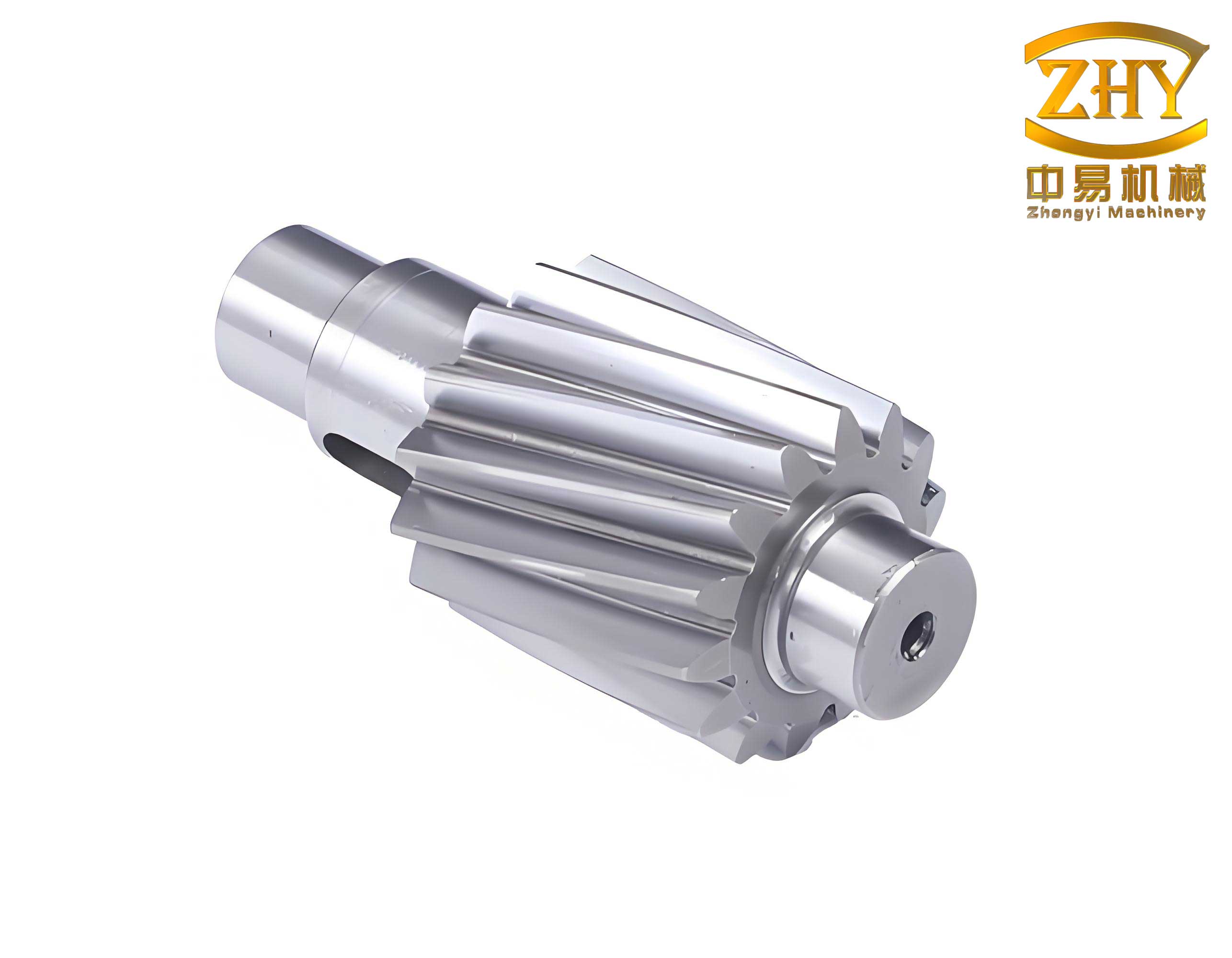
The static analysis of gear shafts begins with the creation of a finite element model. We consider a gear shaft made of 40Cr steel, with material properties including a density of 7850 kg/m³, Poisson’s ratio of 0.277, elastic modulus of 2.11e5 MPa, and a yield strength of 785 MPa. For design safety, a factor of safety of 1.7 is applied, resulting in an allowable stress of 461 MPa. The gear shaft structure is simplified by omitting non-essential features like keyways and grooves to focus on core load-bearing regions. Using SOLID45 elements, the model is meshed via a sweeping technique, resulting in 8912 elements and 9641 nodes. This discretization balances computational accuracy and efficiency, as mesh quality directly affects FEA outcomes.
Loading conditions are derived from operational scenarios. The gear shaft experiences radial and axial forces from helical and bevel gears, along with transmitted torque. For instance, radial and axial forces from the helical gear are calculated as 2643 N and 1545 N, respectively, while those from the bevel gear are 7745.915 N and 2912.471 N. The torque is 230700 N·mm. To avoid stress concentrations, these loads are applied as distributed forces and moments. The boundary conditions involve constraints at bearing installation points. The static analysis yields stress and deformation results. According to the fourth strength theory, the equivalent stress (von Mises stress) is computed using the formula:
$$ \sigma_{eq} = \sqrt{\frac{1}{2}[(\sigma_1 – \sigma_2)^2 + (\sigma_2 – \sigma_3)^2 + (\sigma_3 – \sigma_1)^2]} $$
where $\sigma_1$, $\sigma_2$, and $\sigma_3$ are principal stresses. The analysis reveals that the maximum working stress occurs at the shoulder transition between the bevel gear installation and the right bearing seat, with a value of 50.144 MPa, which is well below the allowable stress of 461 MPa. Thus, the static strength of the gear shafts is satisfactory. Deformation analysis shows a maximum displacement of 0.005143 mm at another shoulder location, indicating adequate stiffness. These results confirm that the gear shafts meet design requirements under given loads.
To further explore the influence of structural parameters, we proceed to sensitivity analysis. The goal is to assess how variations in dimensions affect the maximum working stress of gear shafts. We define 11 design variables: six axial parameters ($l_1$ to $l_6$) and five radial parameters ($d_1$ to $d_5$), as illustrated in the gear shaft schematic. Each variable is assigned three levels, forming a 13-factor, three-level orthogonal array (though we have 11 factors, we use a standard table accommodating 13). This design minimizes the number of experiments while capturing interactions. The sensitivity of a function $f(X)$ to a design variable $x_j$ is defined as:
$$ S_j = \frac{\partial f}{\partial x_j} $$
In practice, for discrete levels, we use the range method from orthogonal experiments. The range $R_j$ for factor $j$ is calculated as:
$$ R_j = \max(\bar{y}_{j1}, \bar{y}_{j2}, \bar{y}_{j3}) – \min(\bar{y}_{j1}, \bar{y}_{j2}, \bar{y}_{j3}) $$
where $\bar{y}_{jk}$ is the average response for factor $j$ at level $k$. A larger $R_j$ indicates greater influence. For two-level designs, sensitivity can be approximated as $|S_j| = 2|R_j| / |x_{j1} – x_{j2}|$, but here we focus on range analysis. The steps include: (1) identifying target function (maximum stress) and design variables, (2) selecting an orthogonal table and setting levels, (3) conducting experiments via FEA, (4) computing averages and ranges, and (5) determining parameter sensitivity and monotonicity.
For our gear shafts, the factor levels are detailed in Table 1. We perform 27 experimental runs according to the orthogonal array, each time rebuilding the FEA model with specified dimensions and recording the maximum stress. The results are compiled in Table 2, showing stress values in MPa for each combination. From this data, we calculate the mean stress for each factor at each level and the corresponding ranges. The analysis reveals that parameter $l_1$ (an axial dimension) has the highest range, meaning it most significantly affects the static stress of gear shafts. This is followed by $d_4$ and $d_5$, while $d_2$ has the least impact. The order of sensitivity is: $l_1$, $d_5$, $d_4$, $l_6$, $l_5$, $l_3$, $l_2$, $l_4$, $d_1$, $d_3$, $d_2$. This ranking guides designers in prioritizing parameters during optimization of gear shafts.
| Factor | $l_1$ | $l_2$ | $l_3$ | $l_4$ | $l_5$ | $l_6$ | $d_1$ | $d_2$ | $d_3$ | $d_4$ | $d_5$ |
|---|---|---|---|---|---|---|---|---|---|---|---|
| Level 1 | 18 | 36 | 53 | 116.25 | 176.25 | 208.75 | 43 | 53 | 69.52 | 50 | 56 |
| Level 2 | 20 | 38 | 55 | 118.25 | 178.25 | 210.75 | 45 | 55 | 71.52 | 52 | 58 |
| Level 3 | 22 | 40 | 57 | 120.25 | 180.25 | 212.75 | 47 | 57 | 73.52 | 54 | 60 |
| Run | $l_1$ | $l_2$ | $l_3$ | $l_4$ | $l_5$ | $l_6$ | $d_1$ | $d_2$ | $d_3$ | $d_4$ | $d_5$ | Stress |
|---|---|---|---|---|---|---|---|---|---|---|---|---|
| 1 | 18 | 36 | 53 | 116.25 | 176.25 | 208.75 | 43 | 53 | 69.52 | 50 | 56 | 86.461 |
| 2 | 18 | 36 | 53 | 116.25 | 178.25 | 210.75 | 45 | 55 | 71.52 | 52 | 58 | 51.379 |
| 3 | 18 | 36 | 53 | 116.25 | 180.25 | 212.75 | 47 | 57 | 73.52 | 54 | 60 | 46.345 |
| 4 | 18 | 38 | 55 | 118.25 | 176.25 | 208.75 | 43 | 55 | 71.52 | 52 | 60 | 51.375 |
| 5 | 18 | 38 | 55 | 118.25 | 178.25 | 210.75 | 45 | 57 | 73.52 | 54 | 56 | 49.03 |
| 6 | 18 | 38 | 55 | 118.25 | 180.25 | 212.75 | 47 | 53 | 69.52 | 50 | 58 | 72.43 |
| 7 | 18 | 40 | 57 | 120.25 | 176.25 | 208.75 | 43 | 57 | 73.52 | 54 | 58 | 57.735 |
| 8 | 18 | 40 | 57 | 120.25 | 178.25 | 210.75 | 45 | 53 | 69.52 | 50 | 60 | 57.311 |
| 9 | 18 | 40 | 57 | 120.25 | 180.25 | 212.75 | 47 | 55 | 71.52 | 52 | 56 | 54.675 |
| 10 | 20 | 36 | 55 | 120.25 | 176.25 | 210.75 | 47 | 53 | 71.52 | 54 | 56 | 105.154 |
| 11 | 20 | 36 | 55 | 120.25 | 178.25 | 212.75 | 43 | 55 | 73.52 | 50 | 58 | 54.337 |
| 12 | 20 | 36 | 55 | 120.25 | 180.25 | 208.75 | 45 | 57 | 69.52 | 52 | 60 | 51.51 |
| 13 | 20 | 38 | 57 | 116.25 | 176.25 | 210.75 | 47 | 55 | 73.52 | 50 | 60 | 74.142 |
| 14 | 20 | 38 | 57 | 116.25 | 178.25 | 212.75 | 43 | 57 | 69.52 | 52 | 56 | 52.326 |
| 15 | 20 | 38 | 57 | 116.25 | 180.25 | 208.75 | 45 | 53 | 71.52 | 54 | 58 | 93.465 |
| 16 | 20 | 40 | 53 | 118.25 | 176.25 | 210.75 | 47 | 57 | 69.52 | 52 | 58 | 56.381 |
| 17 | 20 | 40 | 53 | 118.25 | 178.25 | 212.75 | 43 | 53 | 71.52 | 54 | 60 | 100.659 |
| 18 | 20 | 40 | 53 | 118.25 | 180.25 | 208.75 | 45 | 55 | 73.52 | 50 | 56 | 136.395 |
| 19 | 22 | 36 | 57 | 118.25 | 176.25 | 212.75 | 45 | 53 | 73.52 | 52 | 56 | 50.805 |
| 20 | 22 | 36 | 57 | 118.25 | 178.25 | 208.75 | 47 | 55 | 69.52 | 54 | 58 | 47.521 |
| 21 | 22 | 36 | 57 | 118.25 | 180.25 | 210.75 | 43 | 57 | 71.52 | 50 | 60 | 54.627 |
| 22 | 22 | 38 | 53 | 120.25 | 176.25 | 212.75 | 45 | 55 | 69.52 | 54 | 60 | 48.806 |
| 23 | 22 | 38 | 53 | 120.25 | 178.25 | 208.75 | 47 | 57 | 71.52 | 50 | 56 | 67.19 |
| 24 | 22 | 38 | 53 | 120.25 | 180.25 | 210.75 | 43 | 53 | 73.52 | 52 | 58 | 51.776 |
| 25 | 22 | 40 | 55 | 116.25 | 176.25 | 212.75 | 45 | 57 | 71.52 | 50 | 58 | 56.277 |
| 26 | 22 | 40 | 55 | 116.25 | 178.25 | 208.75 | 47 | 53 | 73.52 | 52 | 60 | 53.056 |
| 27 | 22 | 40 | 55 | 116.25 | 180.25 | 210.75 | 43 | 55 | 69.52 | 54 | 56 | 58.161 |
From Table 2, we compute the mean stress for each factor at each level, as shown in Table 3. The range values are derived, highlighting the sensitivity ranking. For instance, for factor $l_1$, the means at levels 1, 2, and 3 are 58.527 MPa, 80.446 MPa, and 54.247 MPa, respectively, giving a range of 26.199 MPa—the highest among all factors. This underscores the critical role of $l_1$ in governing the stress behavior of gear shafts. Similarly, for $d_4$, the means are 73.241 MPa, 52.547 MPa, and 67.431 MPa, with a range of 20.694 MPa, indicating substantial influence. These findings are pivotal for design optimization, as tweaking high-sensitivity parameters can lead to significant improvements in the performance of gear shafts.
| Factor | Mean Level 1 | Mean Level 2 | Mean Level 3 | Range $R_j$ |
|---|---|---|---|---|
| $l_1$ | 58.527 | 80.446 | 54.247 | 26.199 |
| $l_2$ | 60.864 | 62.282 | 70.072 | 9.208 |
| $l_3$ | 71.710 | 61.219 | 60.290 | 11.420 |
| $l_4$ | 63.512 | 68.803 | 60.904 | 7.899 |
| $l_5$ | 65.237 | 59.201 | 68.781 | 9.580 |
| $l_6$ | 71.594 | 61.996 | 59.629 | 11.965 |
| $d_1$ | 63.051 | 66.069 | 64.099 | 3.018 |
| $d_2$ | 74.569 | 64.088 | 54.562 | 20.007 |
| $d_3$ | 58.950 | 70.533 | 63.736 | 11.583 |
| $d_4$ | 73.241 | 52.547 | 67.431 | 20.694 |
| $d_5$ | 73.355 | 60.145 | 59.719 | 13.636 |
The sensitivity analysis can be further quantified using derivative-based approaches. For continuous variables, the sensitivity $S_j$ can be approximated from the orthogonal data. Assuming a linear relationship, we can estimate partial derivatives. For example, for $l_1$, with levels 18, 20, and 22 mm, and mean stresses as above, the sensitivity around the mid-level can be computed using finite differences. The formula for central difference is:
$$ S_{l_1} \approx \frac{f(l_1 + \Delta l) – f(l_1 – \Delta l)}{2\Delta l} $$
where $\Delta l = 2$ mm. Using mean stresses at levels 1 and 3, we get $S_{l_1} \approx (54.247 – 58.527) / (22 – 18) = -1.07$ MPa/mm. This negative value suggests that increasing $l_1$ decreases stress, which aligns with the range analysis showing lower stress at higher $l_1$ levels for some runs. However, the non-monotonic trend in means indicates complex interactions, typical in gear shafts due to their geometry. Such insights are valuable for iterative design refinement.
Beyond static analysis, the dynamic behavior of gear shafts also warrants attention, but here we focus on static characteristics. The finite element method provides a robust framework for simulating gear shafts under load. The governing equation for static FEA is:
$$ [K]\{u\} = \{F\} $$
where $[K]$ is the global stiffness matrix, $\{u\}$ is the displacement vector, and $\{F\}$ is the force vector. For gear shafts, material nonlinearities may arise, but for 40Cr steel in the elastic regime, linear analysis suffices. The stress is then derived from displacements using strain-displacement relations and Hooke’s law:
$$ \{\sigma\} = [D]\{\epsilon\} $$
with $[D]$ as the elasticity matrix and $\{\epsilon\}$ as the strain vector. In our FEA, these computations are automated, but understanding them helps interpret results. For instance, high stress concentrations at shoulder transitions are expected due to geometric discontinuities, reinforcing the need for fillets or gradual changes in gear shafts.
The orthogonal experimental method, while efficient, has limitations. It assumes factor independence, which may not hold for intricately coupled gear shafts parameters. Advanced techniques like response surface methodology or variance-based sensitivity analysis could complement this. Nevertheless, for preliminary design, orthogonal arrays offer a pragmatic balance. In our case, the L27 array with 11 factors and 3 levels provides 27 runs, each simulating gear shafts under varied dimensions. The computational cost is manageable, and the results are statistically meaningful. The range analysis simplifies decision-making, pointing designers toward critical parameters.
In practice, the design of gear shafts involves trade-offs between strength, stiffness, weight, and manufacturability. The sensitivity analysis informs these trade-offs. For example, since $l_1$ has high sensitivity, adjusting it can reduce stress without major weight increase. Conversely, $d_2$ has low sensitivity, allowing more flexibility in its specification. This is crucial for mass production of gear shafts, where tolerance control impacts cost. Moreover, the static analysis confirms that even with dimensional variations, the maximum stress remains within safe limits, validating the robustness of the initial design for gear shafts.
To generalize, the methodologies applied here—FEA and orthogonal sensitivity analysis—are transferable to other shaft-like components. For instance, in automotive or aerospace applications, similar approaches can optimize drive shafts or rotor shafts. The key is to adapt loading conditions and constraints. For gear shafts specifically, the inclusion of gear forces adds complexity, but the principles remain. Future work could explore fatigue analysis or thermal effects, but static characteristics form the foundation.
In conclusion, this study underscores the importance of comprehensive analysis for gear shafts. Through finite element static analysis, we verified that the gear shafts meet strength and stiffness requirements under operational loads. The maximum working stress is 50.144 MPa, below the allowable 461 MPa, and deformation is minimal. Sensitivity analysis via orthogonal experiments revealed that axial parameter $l_1$ most influences stress, followed by radial parameters $d_4$ and $d_5$, while $d_2$ has the least effect. These insights enable targeted optimization, improving design efficiency for gear shafts. As mechanical systems evolve, such analytical rigor will continue to ensure the reliability and performance of gear shafts in diverse engineering applications.