
The paradigm of mechanical design has progressively shifted from deterministic methods towards probabilistic approaches, with reliability design emerging as a cornerstone of modern engineering practice. Often termed mechanical probability design, this methodology fundamentally redefines how components are conceived and analyzed. Traditional mechanical design typically treats loads, material strengths, and dimensions as fixed, deterministic values, applying safety factors to account for uncertainties. In stark contrast, reliability design explicitly acknowledges and quantifies the inherent randomness in all aspects of a component’s lifecycle.
The core distinctions of reliability design are profound. Firstly, it recognizes that both the stress (S) acting on a component and its strength (R) to withstand that stress are not single values but random variables. These variables are characterized by their statistical distributions, considering not only the mean (average) values but, crucially, their dispersion or variability, quantified using parameters like standard deviation. Solutions are derived using probability and statistical methods. Secondly, this approach accepts that any mechanical design carries a finite probability of failure. The design process allows engineers to explicitly specify and control this failure probability or its complement, the reliability (R). By incorporating the statistical nature of all design parameters, reliability design offers a more realistic reflection of a component’s actual operational conditions. Consequently, thirdly, it is widely regarded as a more rational and efficient methodology compared to the traditional safety factor approach. While a global safety factor often leads to overly conservative, and thus heavier and more expensive, designs, reliability design aims for a “right-sized” component that meets a specified reliability target. This optimization can lead to significant savings in material, weight, and manufacturing cost while maintaining or even improving performance confidence.
Empirical evidence from reliability theory and mechanical engineering practice consistently shows that material properties, operational loads, environmental conditions, and the very processes leading to failure are inherently stochastic. For critical components like gear shafts, parameters such as bending stress, torsional stress, material yield strength, fatigue endurance limit, and even geometric dimensions exhibit natural scatter and are best described by probability distributions.
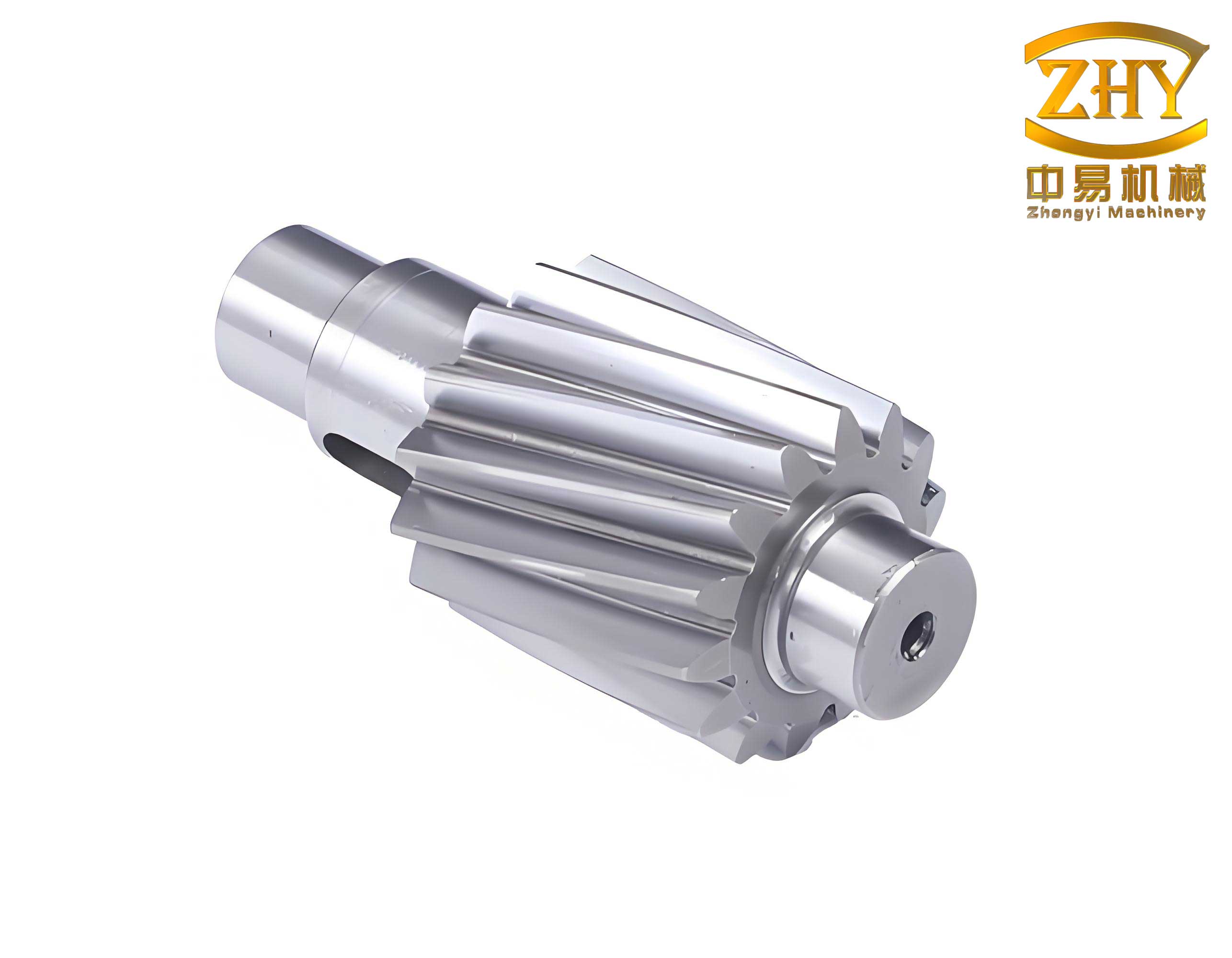
Fundamental Theory of Reliability Design and Reliability Computation
1.1 Core Theoretical Analysis
The fundamental premise of reliability design rests on the concept of the stress-strength interference model. In this model, the strength of a component, denoted as \( S \), is a random variable with a probability density function (PDF) \( f_S(s) \). Simultaneously, the stress experienced by the component, denoted as \( L \), is another random variable with PDF \( g_L(l) \). The “reliability” of the component is defined as the probability that its strength exceeds the applied stress. Mathematically, this is expressed as the probability that the difference \( Z = S – L \) is greater than zero:
$$ R = P(S > L) = P( (S – L) > 0 ) = P(Z > 0) $$
When the PDFs of stress and strength are plotted on the same axis, they may overlap or “interfere,” as illustrated in the model. The area of this interference region represents situations where the applied stress exceeds the component’s strength, i.e., the probability of failure \( F \). The reliability is thus \( R = 1 – F \).
To compute this, consider a narrow band of stress of width \( dL \) centered at a value \( L = L_0 \). The probability of the stress lying in this interval is approximately \( g_L(L_0) \, dL \). For this specific stress level, failure occurs if the strength \( S \) is less than \( L_0 \). The conditional probability of this event is \( \int_{0}^{L_0} f_S(s) \, ds \). Since stress and strength are independent random variables, the total probability of failure is found by integrating over all possible stress levels:
$$ F = P(S \le L) = \int_{0}^{\infty} \left[ \int_{0}^{l} f_S(s) \, ds \right] g_L(l) \, dl $$
Therefore, the general expression for reliability is:
$$ R = 1 – F = \int_{0}^{\infty} \left[ \int_{l}^{\infty} f_S(s) \, ds \right] g_L(l) \, dl $$
This integral provides a universal framework for reliability calculation, contingent upon knowing the specific distribution forms of \( f_S(s) \) and \( g_L(l) \).
1.2 Reliability Calculation for Normally Distributed Stress and Strength
Extensive experimental data in mechanical engineering suggests that for many materials and loading conditions, both strength and stress can be reasonably modeled by the normal (Gaussian) distribution. This assumption greatly simplifies analysis. Let strength \( S \) follow a normal distribution with mean \( \mu_S \) and standard deviation \( \sigma_S \), and stress \( L \) follow a normal distribution with mean \( \mu_L \) and standard deviation \( \sigma_L \):
$$ f_S(s) = \frac{1}{\sigma_S \sqrt{2\pi}} \exp\left[-\frac{1}{2}\left(\frac{s – \mu_S}{\sigma_S}\right)^2\right] $$
$$ g_L(l) = \frac{1}{\sigma_L \sqrt{2\pi}} \exp\left[-\frac{1}{2}\left(\frac{l – \mu_L}{\sigma_L}\right)^2\right] $$
A fundamental result from probability theory states that the linear combination of independent normal variables is also normally distributed. Therefore, the safety margin \( Z = S – L \) is normally distributed with the following parameters:
$$ \mu_Z = \mu_S – \mu_L $$
$$ \sigma_Z = \sqrt{\sigma_S^2 + \sigma_L^2} $$
The PDF of \( Z \) is:
$$ h_Z(z) = \frac{1}{\sigma_Z \sqrt{2\pi}} \exp\left[-\frac{1}{2}\left(\frac{z – \mu_Z}{\sigma_Z}\right)^2\right] $$
Failure occurs when \( Z \le 0 \). The reliability is the probability that \( Z > 0 \):
$$ R = P(Z > 0) = \int_{0}^{\infty} h_Z(z) \, dz $$
This integral is evaluated by transforming to the standard normal variable \( t = (z – \mu_Z)/\sigma_Z \). When \( z = 0 \), \( t = -\mu_Z / \sigma_Z \). When \( z \to \infty \), \( t \to \infty \). Thus,
$$ R = \int_{-\mu_Z/\sigma_Z}^{\infty} \phi(t) \, dt = 1 – \Phi\left(-\frac{\mu_Z}{\sigma_Z}\right) $$
where \( \phi(t) \) is the standard normal PDF and \( \Phi \) is its cumulative distribution function (CDF). Due to the symmetry of the normal distribution, this simplifies to the crucial Reliability Index or Coupling Equation:
$$ R = \Phi(\beta) $$
where
$$ \beta = \frac{\mu_Z}{\sigma_Z} = \frac{\mu_S – \mu_L}{\sqrt{\sigma_S^2 + \sigma_L^2}} $$
The term \( \beta \) is known as the reliability index or coupling coefficient. It directly links the statistical parameters of stress and strength to the component’s reliability. Given \( \beta \), the reliability \( R \) can be obtained directly from standard normal distribution tables. This elegant equation is a workhorse in mechanical reliability design for components like gear shafts when normal distribution assumptions hold.
| Aspect | Traditional Deterministic Design | Probabilistic Reliability Design |
|---|---|---|
| Core Philosophy | Use single, worst-case values for stress and strength. | Treat stress and strength as random variables with distributions. |
| Safety Measure | Global Safety Factor \( n = \mu_S / \mu_L \) (deterministic). | Reliability \( R \) or Probability of Failure \( F \) (probabilistic). |
| Variability Consideration | Implicitly accounted for by an often arbitrary safety factor. | Explicitly modeled via standard deviations \( \sigma_S \) and \( \sigma_L \). |
| Design Outcome | Can be overly conservative or, in rare cases, non-conservative. | Aims for optimal design meeting a specific, quantifiable reliability target. |
| Information Requirement | Mean values of load and strength. | Mean and variance of load, strength, geometry, etc. |
| Application to Gear Shafts | Calculates diameter based on max load and min strength with a factor. | Calculates diameter distribution to ensure \( P(S > L) \ge R_{target} \). |
Analysis of Gear Shaft Loading and Failure Modes
Gear shafts are critical power transmission elements, subject to complex multiaxial stress states. A comprehensive reliability analysis must begin with a thorough understanding of their operational loads and potential failure mechanisms.
2.1 Load State Analysis
A typical gear shaft transmits torque while supporting radial loads from gears, leading to combined bending and torsion. At any critical cross-section (often at shoulders, keyways, or press-fit locations), the stress state is defined by:
– Bending Stress (\( \sigma_b \)): Caused by transverse loads. For rotating gear shafts, this is often a fully reversed (symmetrical) cyclic stress.
– Torsional Shear Stress (\( \tau \)): Caused by transmitted torque. This is often a repeated or pulsating (zero-to-max) cyclic stress.
The combined stress must be evaluated using an appropriate failure theory. For ductile materials like alloy steels commonly used for gear shafts, the Von Mises or distortion energy theory is applied to find an equivalent alternating (von Mises) stress. Furthermore, stress concentrations at geometric discontinuities (e.g., fillets, keyways) significantly reduce fatigue strength and are accounted for by a fatigue stress concentration factor \( K_f \). The loading on a gear shaft is therefore characterized by statistical parameters for bending moment \( M \), torque \( T \), and the stress concentration factor.
2.2 Failure Mode and Fatigue Analysis
The dominant failure mode for dynamically loaded gear shafts is fatigue fracture. A classic fatigue fracture surface exhibits distinct zones:
1. Crack Initiation Site(s): Often at a surface defect, sharp corner, or inclusion.
2. Fatigue Crack Growth Region: Characterized by progressive “beach marks” or “clamshell” patterns indicating successive positions of the crack front during load cycles.
3. Final Fracture Zone: The remaining cross-section fails by overload (ductile or brittle fracture) when the crack reduces the effective area to a critical size.
The presence of a large fatigue growth zone relative to the final fracture zone indicates high-cycle fatigue, where stresses were predominantly below the yield strength. The initiation of cracks at stress concentrators underscores the critical importance of detailed design (fillet radii, surface finish) and accurate modeling of stress gradients in the reliability assessment of gear shafts. The fatigue life \( N \) itself is a random variable, often following a log-normal or Weibull distribution.
Reliability-Based Design Procedure for a Gear Shaft
This section demonstrates the application of reliability theory to the design of a gear shaft, contrasting static and fatigue strength approaches. The design variable (shaft diameter \( d \)) will be determined to meet a specified reliability target.
3.1 Establishing Design Parameters and Reliability Target
Consider a power transmission gear shaft made of quenched and tempered 40Cr alloy steel. The shaft experiences combined cyclic bending and torsion. From load analysis, the statistical parameters for the critical section are estimated. We define a target reliability \( R \) and a corresponding reliability index \( \beta \) from the standard normal table. A “design factor” \( n_d \) (analogous to but distinct from a safety factor) may be applied to the mean stress for an additional safety margin in the calculation setup.
| Parameter | Symbol | Mean Value | Coefficient of Variation (COV) | Notes / Calculation |
|---|---|---|---|---|
| Target Reliability | \( R \) | – | – | Set to 0.99 for critical component. |
| Reliability Index | \( \beta \) | \( \Phi^{-1}(0.99) \) | – | \( \beta = 2.326 \) from standard normal table. |
| Design (Margin) Factor | \( n_d \) | 1.25 | – | Applied to mean stress in the coupling equation. |
| Material Yield Strength | \( S_y \) | \( \mu_{S_y} = 540 \, \text{MPa} \) | \( V_{S_y} = 0.07 \) | 40Cr Steel, quenched & tempered. \( \sigma_{S_y} = V_{S_y} \cdot \mu_{S_y} \). |
| Material Ultimate Strength | \( S_u \) | \( \mu_{S_u} = 735 \, \text{MPa} \) | \( V_{S_u} = 0.05 \) | |
| Material Fatigue Endurance Limit | \( S_e’ \) | \( \mu_{S_e’} \approx 0.5 \mu_{S_u} \) | \( V_{S_e’} = 0.08 \) | Estimated for polished specimen. |
| Fatigue Stress Conc. Factor | \( K_f \) | \( \mu_{K_f} = 2.0 \) | \( V_{K_f} = 0.05 \) | Depends on geometry (fillet radius). |
| Bending Moment (Alternating) | \( M_a \) | \( \mu_{M} = 7.5 \, \text{kN·m} \) | \( V_{M} = 0.15 \) | From load spectrum analysis. |
| Torque (Mid-range/Static) | \( T_m \) | \( \mu_{T} = 7.8 \, \text{kN·m} \) | \( V_{T} = 0.10 \) | |
| Stress COV | \( V_{\sigma} \) | 0.08 | – | Assumed for calculated stress. |
3.2 Design for Static Yield Strength (Non-Cyclic Overload)
This check ensures the gear shaft does not yield under peak loads (e.g., startup, shock). The Von Mises stress is used. The mean strength for static yield is the mean yield strength \( \mu_{S_y} \). The mean Von Mises stress \( \mu_{\sigma_{vm}} \) at the critical diameter \( d \) is:
$$ \mu_{\sigma_{vm}} = \frac{\sqrt{ (\mu_{\sigma_b})^2 + 3(\mu_{\tau})^2 }}{n_d} $$
where \( \mu_{\sigma_b} = \frac{32 \mu_M}{\pi d^3} \) and \( \mu_{\tau} = \frac{16 \mu_T}{\pi d^3} \). The standard deviations are approximated by propagating uncertainties: \( \sigma_{\sigma_{vm}} \approx V_{\sigma} \cdot \mu_{\sigma_{vm}} \), and \( \sigma_{S_y} = V_{S_y} \cdot \mu_{S_y} \). The coupling equation becomes:
$$ \beta = \frac{\mu_{S_y} – \mu_{\sigma_{vm}}}{\sqrt{\sigma_{S_y}^2 + \sigma_{\sigma_{vm}}^2}} $$
This equation is solved iteratively for the diameter \( d \) that yields \( \beta \ge 2.326 \). For the given parameters, this results in:
$$ d_{static} \ge 83.4 \, \text{mm} $$
3.3 Design for Fatigue Strength (Infinite Life)
This is the governing design criterion for rotating gear shafts under cyclic loads. We apply the modified Goodman criterion in a stochastic context. The mean fully corrected endurance limit \( \mu_{S_e} \) is:
$$ \mu_{S_e} = \frac{\mu_{S_e’} \cdot C_{load} \cdot C_{size} \cdot C_{surf} \cdot C_{temp} \cdot C_{reliab}}{\mu_{K_f}} $$
where various \( C \) factors account for loading type, size, surface finish, temperature, and a deterministic reliability correction (different from probabilistic \( R \)). The mean alternating stress \( \mu_{\sigma_a} \) is primarily from bending: \( \mu_{\sigma_a} = \frac{32 \mu_M}{\pi d^3} \). The mean midrange Von Mises stress \( \mu_{\sigma_m} \) is from the steady torsion component: \( \mu_{\sigma_m} = \sqrt{3} \cdot \mu_{\tau} = \sqrt{3} \cdot \frac{16 \mu_T}{\pi d^3} \).
The stochastic modified Goodman relation defines an equivalent alternating strength \( \mu_{S_{eq}} \):
$$ \mu_{S_{eq}} = \frac{\mu_{\sigma_a}}{1 – \frac{\mu_{\sigma_m}}{\mu_{S_u}}} $$
This equivalent strength \( S_{eq} \) is the random variable representing the component’s fatigue strength under the given mean stress. Its standard deviation \( \sigma_{S_{eq}} \) is derived from error propagation of all contributing variables. The mean and standard deviation of the applied alternating stress are \( \mu_{\sigma_a} \) and \( \sigma_{\sigma_a} \approx V_{\sigma} \cdot \mu_{\sigma_a} \). The coupling equation for fatigue is:
$$ \beta_{fatigue} = \frac{\mu_{S_{eq}} – \mu_{\sigma_a}}{\sqrt{\sigma_{S_{eq}}^2 + \sigma_{\sigma_a}^2}} $$
Solving this more complex equation for \( d \) such that \( \beta_{fatigue} \ge 2.326 \) yields a larger, governing diameter:
$$ d_{fatigue} \ge 99.3 \, \text{mm} $$
Therefore, the design must be based on the fatigue criterion, selecting a standard diameter of \( d = 100 \, \text{mm} \) for the critical section of the gear shaft.
| Design Criterion | Calculated Min. Diameter (mm) | Governing Reliability Index \( \beta \) | Implied Reliability \( R \) | Notes |
|---|---|---|---|---|
| Static Yield | 83.4 | 2.326 | 0.990 | Non-cyclic overload check. |
| Fatigue (Infinite Life) | 99.3 | 2.326 | 0.990 | Governs for rotating shaft. |
| Final Design Selection | 100.0 | > 2.326 | > 0.990 | Standard diameter chosen. |
3.4 Sensitivity and Alternative Design Strategies
The analysis reveals that fatigue strength is the limiting factor. If increasing the diameter is not feasible, reliability can be enhanced by modifying other parameters in the coupling equation, thereby increasing \( \beta \). Key strategies for gear shafts include:
– Reduce Mean Stress (\( \mu_L \)): Optimize load sharing, use smoother gear profiles, improve system dynamics.
– Reduce Stress Variability (\( \sigma_L \)): Implement better control over operational loads and conditions.
– Increase Mean Strength (\( \mu_S \)): Use a higher-grade material, or more effective heat treatment (e.g., induction hardening of fillets).
– Reduce Strength Variability (\( \sigma_S \)): Employ stricter material quality control and process standardization.
– Increase Fatigue Strength Specifically: The most effective lever is often reducing the stress concentration factor \( K_f \). This can be achieved by:
1. Increasing Fillet Radii: A larger radius dramatically decreases \( K_t \) and thus \( K_f \).
2. Improving Surface Finish: Grinding or polishing the critical region increases the material’s effective endurance limit.
3. Introducing Compressive Residual Stresses: Processes like shot peening or roller burnishing induce surface compressive stresses, effectively increasing \( \mu_{S_e} \) and reducing \( \sigma_{S_e} \).
Applying these measures would allow for a smaller, lighter gear shaft to achieve the same reliability target, or significantly boost the reliability of an existing shaft geometry.
Advanced Considerations and Conclusions
The preceding analysis assumes normal distributions for simplicity. In practice, other distributions like the Weibull distribution (excellent for modeling fatigue life and strength of brittle materials) or the log-normal distribution (often used for fatigue strength and crack growth rates) may be more appropriate. The general interference integral \( R = \int_{0}^{\infty} \left[ \int_{l}^{\infty} f_S(s) \, ds \right] g_L(l) \, dl \) remains valid, but numerical integration or simulation techniques like Monte Carlo analysis are required for solution. For gear shafts in particular, modeling the distribution of surface defects or inclusions that initiate fatigue cracks might necessitate a Weibull-based weakest-link theory.
Furthermore, a comprehensive reliability design of a gear shaft extends beyond the diameter calculation. It involves the probabilistic analysis of deflections (to ensure gear mesh alignment), critical speeds (to avoid resonance), and wear life. The reliability of the entire power transmission system is a function of the reliability of its individual components, including gear shafts, bearings, and gears, and their interactions.
In conclusion, the reliability-based design methodology provides a powerful, rational, and quantitative framework for designing mechanical components like gear shafts. By moving beyond deterministic safety factors to explicitly model the uncertainties in stress, strength, and geometry, it enables engineers to:
1. Quantify Risk: Specify and verify a precise probability of failure or success.
2. Optimize Design: Achieve lighter, more cost-effective designs without compromising safety.
3. Make Informed Decisions: Evaluate the impact of material choices, manufacturing tolerances, and operational conditions on component life.
4. Diagnose Failures: Understand the probabilistic contributors to field failures and implement targeted improvements.
The application of stress-strength interference theory, culminating in the coupling equation for normally distributed variables, offers a direct and insightful design tool. When applied to critical rotating elements like gear shafts, it shifts the design philosophy from “Is the safety factor high enough?” to “What is the probability this shaft will survive its intended service life?” This probabilistic mindset is essential for advancing the safety, efficiency, and innovation of modern mechanical systems.