
In mechanical transmission systems, screw gears, particularly double lead screw gears, play a pivotal role due to their ability to provide high reduction ratios and precise motion control in applications such as indexing mechanisms and reducers. The double lead design, where the left and right tooth surfaces have different leads, allows for axial adjustment to minimize backlash, enhancing transmission accuracy without altering the center distance. However, achieving precise three-dimensional models of these screw gears has been a longstanding challenge in computer-aided design (CAD). Traditional modeling methods often rely on simplified approximations, leading to inaccuracies that can affect subsequent analyses like finite element simulation and CNC machining. In this paper, I explore a novel and accurate modeling methodology for double lead screw gears based on the UG software, leveraging the principles of gear generation and vector algebra to ensure fidelity to actual manufacturing processes. This approach is applicable to various screw gear types with different tooth profiles and lead variations, offering a robust foundation for advanced engineering applications.
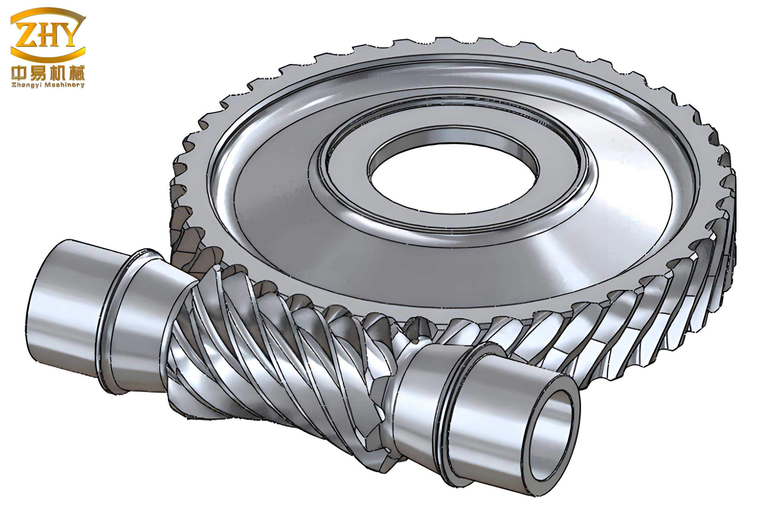
The core of this method lies in simulating the cutting process: the contact line between the cutting tool and the screw gear blank is used to generate helical paths for each tooth surface, forming precise spiral surfaces that define the gear tooth geometry. By conjugating these surfaces, the mating gear tooth profile is derived, resulting in an accurate digital twin. Throughout this discussion, I will emphasize the term “screw gear” to underscore the focus on helical motion and gear interaction. The integration of mathematical formulations, tabular data, and practical CAD steps will provide a holistic guide for engineers and designers. To visually complement the text, I include an illustration of a typical screw gear assembly, which highlights the intricate helical structure central to this study.
The significance of precise screw gear modeling cannot be overstated. In industries ranging from aerospace to robotics, even minor deviations in gear geometry can lead to performance issues like noise, vibration, and premature wear. Double lead screw gears, with their unique ability to control backlash through axial displacement, require especially careful modeling to capture the nuanced differences between left and right tooth surfaces. Common screw gear types include Archimedean, involute, and extended involute profiles, each with distinct mathematical representations. The Archimedean screw gear, for instance, has a straight axial tooth profile, making it relatively easier to model via linear sweeps. However, involute and extended involute screw gears involve complex curves that are not easily described by simple equations, necessitating a more sophisticated approach. My methodology addresses this by deriving tooth surfaces from fundamental cutting kinematics, ensuring accuracy across all screw gear variants.
To understand the modeling process, it is essential to first delve into the working and manufacturing principles of double lead screw gears. In a double lead screw gear pair, the screw gear (worm) has two different leads on its left and right flanks, while the lead on each side remains constant. This design results in a varying axial tooth thickness along the screw gear’s length, allowing for adjustable meshing clearance. The manufacturing typically involves using a straight-edged cutting tool, such as a lathe tool, where the tool’s orientation relative to the screw gear blank determines the resulting tooth profile. For example, when the tool edge is placed in the axial plane, an Archimedean screw gear is produced; if tilted at the helix angle in the normal plane, an extended involute screw gear results. This cutting action can be mathematically represented as a helical motion of the tool contact line, forming a spiral surface. By capturing this motion in UG, I can replicate the exact tooth geometry as it would be machined in reality.
The mathematical foundation for this modeling approach relies on vector algebra to describe helical transformations. Consider a vector $\mathbf{r}(x, y, z)$ in a coordinate system $O-ijk$. When this vector rotates around the $k$-axis by an angle $\phi$ and simultaneously translates along the $k$-axis by a distance $p\phi$, where $p$ is the lead parameter (positive for right-hand helices, negative for left-hand helices), its new position $\mathbf{r}'(x’, y’, z’)$ is given by the helical motion equation:
$$ \begin{bmatrix} x’ \\ y’ \\ z’ \end{bmatrix} = \begin{bmatrix} \cos \phi_k & -\sin \phi_k & 0 \\ \sin \phi_k & \cos \phi_k & 0 \\ 0 & 0 & 1 \end{bmatrix} \begin{bmatrix} x \\ y \\ z \end{bmatrix} + \begin{bmatrix} 0 \\ 0 \\ p\phi \end{bmatrix} $$
This transformation generates a helical path. If the vector $\mathbf{r}$ represents a point on the tool contact line, then as $\phi$ varies, the locus of these points forms a spiral surface—the tooth flank of the screw gear. For a double lead screw gear, separate transformations are applied for the left and right flanks with distinct lead parameters $p_z$ and $p_y$. The general form for a spiral surface derived from a parametric curve $\mathbf{r}(t) = [x(t), y(t), z(t)]^T$ is:
$$ \begin{bmatrix} x’ \\ y’ \\ z’ \end{bmatrix} = \begin{bmatrix} \cos \phi & -\sin \phi & 0 \\ \sin \phi & \cos \phi & 0 \\ 0 & 0 & 1 \end{bmatrix} \begin{bmatrix} x(t) \\ y(t) \\ z(t) \end{bmatrix} + \begin{bmatrix} 0 \\ 0 \\ p\phi \end{bmatrix} $$
where $t$ is a parameter along the contact line. This equation is pivotal for generating accurate screw gear models in UG, as it allows for the precise mapping of tool paths into three-dimensional surfaces.
To illustrate the parameter calculations for a double lead screw gear, I consider an extended involute screw gear from a numerical control rotary table mechanism. Key parameters include axial module $m = 1.5 \, \text{mm}$, normal pressure angle $\alpha_{on} = 15^\circ$, number of starts $z_1 = 1$, right-hand helix, left flank axial pitch $t_z = 4.7686 \, \text{mm}$, right flank axial pitch $t_y = 4.6561 \, \text{mm}$, screw gear reference diameter $d_{f1} = 32 \, \text{mm}$, and center distance $A = 76 \, \text{mm}$. The mating gear has $z_2 = 80$ teeth. The following calculations derive essential dimensions for modeling.
First, the nominal axial pitch $t_0$ and pitch difference $\Delta t$ are computed:
$$ t_0 = m\pi = 1.5 \times 3.1416 = 4.7124 \, \text{mm} $$
$$ \Delta t = \frac{t_z – t_y}{2} = \frac{4.7686 – 4.6561}{2} = 0.0563 \, \text{mm} $$
The left and right flank modules are then:
$$ m_z = \frac{t_z}{\pi} = \frac{4.7686}{3.1416} = 1.5179 \, \text{mm} $$
$$ m_y = \frac{t_y}{\pi} = \frac{4.6561}{3.1416} = 1.4821 \, \text{mm} $$
These module differences induce profile shifts. The screw gear pitch diameters for right and left flanks, considering positive and negative shifts, are:
$$ d_{1y} = d_{f1} + \Delta m \cdot z_2 = 33.432 \, \text{mm} \quad \text{(right flank, positive shift)} $$
$$ d_{1z} = d_{f1} – \Delta m \cdot z_2 = 30.568 \, \text{mm} \quad \text{(left flank, negative shift)} $$
where $\Delta m = m_z – m = 0.0179 \, \text{mm}$. The helix angles at these pitch diameters are crucial for spiral generation:
$$ \lambda_y = \arctan\left( \frac{m_y z_1}{d_{1y}} \right) = 2.5384^\circ $$
$$ \lambda_z = \arctan\left( \frac{m_z z_1}{d_{1z}} \right) = 2.8428^\circ $$
Additionally, the axial pressure angles differ due to helix effects:
$$ \alpha_{oay} = \arctan\left( \frac{\tan \alpha_{on}}{\cos \lambda_y} \right) = 15.0117^\circ $$
$$ \alpha_{oaz} = \arctan\left( \frac{\tan \alpha_{on}}{\cos \lambda_z} \right) = 15.0134^\circ $$
For the mating screw gear (worm wheel), key dimensions include reference diameter $d_{f2} = m_n z_2 = 120 \, \text{mm}$, addendum diameter $d_{e2} = 123 \, \text{mm}$, and pitch diameters for each flank: $d_{f2y} = m_y z_2 = 118.568 \, \text{mm}$ and $d_{f2z} = m_z z_2 = 121.432 \, \text{mm}$. The base circle diameters, important for involute geometry, are $d_{oy} = d_{f2y} \cos \alpha_{oay} = 114.5248 \, \text{mm}$ and $d_{oz} = d_{f2z} \cos \alpha_{oaz} = 117.2912 \, \text{mm}$.
To ensure proper meshing, the screw gear length $L$ must account for engagement length $L_\alpha$, process length $L_t$, and adjustment length $L_p$. Calculations based on gear geometry yield:
$$ L_\alpha = \max(e_{y2}, e_{z1}) + \max(e_{y1}, e_{z2}) = 11.9909 \, \text{mm} $$
$$ L_p = \frac{\Delta s}{k_s} = 9.0907 \, \text{mm} \quad \text{(with adjustment amount } \Delta s = 0.2) $$
$$ L_t = 2m\pi = 9.4248 \, \text{mm} $$
$$ L = L_\alpha + L_t + L_p = 30.5064 \, \text{mm} $$
where $e_{y2}, e_{z1}, e_{y1}, e_{z2}$ are engagement limits derived from tooth geometry, and $k_s = (t_z – t_y)/t_0 = 0.02387$ is the thickness increment coefficient. The minimum axial tooth top width $S_a$ and tooth space width $b_{\min}$ are also computed to avoid interference:
$$ S_a = \frac{1}{2} \pi m – \frac{1}{2} L k_s – f_0 m (\tan \alpha_{oaz} + \tan \alpha_{oay}) = 1.1875 \, \text{mm} $$
$$ b_{\min} = \frac{1}{2} \pi m (1 + k_s) – \frac{1}{2} L k_s – (f_0 + c_0) m (\tan \alpha_{oaz} + \tan \alpha_{oay}) = 1.0816 \, \text{mm} $$
These parameters are summarized in Table 1 for clarity, providing a quick reference for designers working with double lead screw gears.
| Parameter | Symbol | Value | Unit |
|---|---|---|---|
| Axial Module | $m$ | 1.5 | mm |
| Normal Pressure Angle | $\alpha_{on}$ | 15 | ° |
| Left Flank Axial Pitch | $t_z$ | 4.7686 | mm |
| Right Flank Axial Pitch | $t_y$ | 4.6561 | mm |
| Pitch Difference | $\Delta t$ | 0.0563 | mm |
| Screw Gear Reference Diameter | $d_{f1}$ | 32 | mm |
| Left Flank Helix Angle | $\lambda_z$ | 2.8428 | ° |
| Right Flank Helix Angle | $\lambda_y$ | 2.5384 | ° |
| Center Distance | $A$ | 76 | mm |
| Mating Gear Teeth | $z_2$ | 80 | – |
| Screw Gear Length | $L$ | 30.5064 | mm |
With these calculations, I proceed to the UG-based modeling of the double lead screw gear. The process begins with defining the coordinate system: the screw gear axis aligns with the Z-axis, and the tooth space centerline at the minimum axial tooth width location defines the X-axis, with origin O at their intersection. For the extended involute screw gear, the tool contact line endpoints in the axial plane are determined. For instance, points A, B, C, D might have coordinates (X1 = 17.5, Z1 = -1.9031), (X2 = 14.2, Z2 = -1.018), (X3 = 17.5, Z3 = 1.903), and (X4 = 14.2, Z4 = 1.0181) in millimeters, representing the left and right edges of the tooth space. These points are treated as vectors from the origin.
In UG NX10, I use the “Expressions” tool under “Tools” to create mathematical formulas for the helical motion. For each endpoint vector, I apply the transformation equation with the respective lead and helix angle. For example, for the left flank with lead $p_z$ and helix angle $\lambda_z$, the helical path for point A is generated using “Law Curve” under “Insert” -> “Curve”, with parametric equations derived from the vector rotation and translation. Similarly, for the right flank with $p_y$ and $\lambda_y$, separate helices are created. This results in four helical curves corresponding to the tooth space boundaries. These curves are then connected with straight lines at their starting ends to form closed loops, which serve as the basis for surface generation.
The next step involves constructing surfaces from these helical curves. Using “Ruled Surface” or “Through Curve Mesh” under “Insert” -> “Mesh Surface”, I create surfaces that represent the tooth flanks. For instance, the surface between the helices of points A and B forms one side of the tooth space. These surfaces are then stitched together using “Sew” under “Insert” -> “Combine” to form a solid representation of the tooth space. This solid is subtracted from the screw gear blank (a cylindrical body) via Boolean operations (“Subtract”) to carve out the tooth space. Repeating this for multiple teeth along the screw gear length, while accounting for the axial variation in tooth thickness, yields the complete double lead screw gear model. To ensure full engagement, I extend the modeling to include 2-3 additional teeth beyond the calculated length $L$.
Table 2 outlines the key UG modeling steps, providing a systematic guide for users aiming to implement this method for screw gear design.
| Step | Action in UG | Description |
|---|---|---|
| 1 | Define Expressions | Create formulas for helix angles, leads, and point coordinates using “Tools” -> “Expressions”. |
| 2 | Generate Helical Curves | Use “Insert” -> “Curve” -> “Law Curve” to produce helices for left and right flanks based on vector transformations. |
| 3 | Close Curve Loops | Draw straight lines to connect helix starts, forming closed boundaries for surface creation. |
| 4 | Create Surfaces | Apply “Ruled Surface” or “Through Curve Mesh” to build spiral surfaces between helical curves. |
| 5 | Stitch Surfaces | Use “Sew” to combine surfaces into a solid tooth space entity. |
| 6 | Boolean Subtraction | Subtract the tooth space solid from the screw gear blank to form gear teeth. |
| 7 | Pattern Teeth | Circularly array the tooth spaces around the axis to complete the screw gear model. |
| 8 | Add Features | Incorporate other details like shafts, fillets, and threads as needed. |
For the mating screw gear (worm wheel), modeling leverages the conjugate action principle. In UG, I use the assembly environment to position the screw gear model relative to the gear blank. Through “WAVE Geometry Linker”, I copy the screw gear tooth surfaces as linked geometry onto the blank. Then, using Boolean “Subtract”, I create tooth spaces in the gear blank. However, these spaces may initially be irregular. To refine them, I extract boundary curves from a representative tooth space using “Insert” -> “Derived Curve” -> “Extract”, then generate a filled surface with “Surface” -> “Fill Surface”. This surface is stitched into a solid tooth space, which is then circularly patterned (e.g., 80 instances for $z_2 = 80$) and merged with the gear blank via Boolean “Intersect” to produce the final gear teeth. This approach ensures accurate conjugation, mimicking the gear hobbing process used in manufacturing.
The advantages of this screw gear modeling method are manifold. Firstly, it is highly accurate because it directly emulates the cutting process, capturing true tooth geometry rather than relying on approximations. This accuracy is critical for subsequent simulations, such as finite element analysis (FEA) for stress distribution or dynamic motion studies. For example, in FEA, precise geometry ensures realistic contact patterns and load sharing between tooth flanks, leading to reliable predictions of gear life and performance. Secondly, the method is versatile, applicable to various screw gear types—Archimedean, involute, or extended involute—by simply adjusting the tool orientation parameters in the vector equations. This flexibility makes it a valuable tool for designers working with diverse screw gear applications, from heavy-duty reducers to precision instruments.
Moreover, the integration of mathematical formulations with UG’s parametric capabilities allows for easy modifications. Design parameters like module, pressure angle, or lead can be updated in the expressions, automatically regenerating the model. This parametricity facilitates optimization studies, where multiple screw gear configurations can be rapidly evaluated to meet specific performance criteria. Additionally, the method supports the design of cutting tools themselves; by treating the contact line as the tool front edge, aspects like relief angles and tool strength can be analyzed to prevent interference and enhance durability during actual machining.
To further illustrate the broad applicability, consider the historical context of screw gear development. Screw gears have evolved from ancient wooden mechanisms to modern high-precision components, with double lead designs emerging in the mid-20th century for backlash control in machine tools and robotics. Today, they are integral in aerospace actuators, medical devices, and renewable energy systems. For instance, in wind turbine yaw drives, double lead screw gears provide reliable positioning under varying loads, and accurate modeling is essential for ensuring longevity in harsh environments. By employing the UG-based method, engineers can simulate wear patterns or thermal effects, leading to improved material selection and lubrication strategies.
In comparison to traditional modeling techniques, such as sweeping a 2D profile along a helix, this approach eliminates common inaccuracies. For involute screw gears, the axial tooth profile is not a simple curve; sweeping an involute along a helix does not yield the correct spiral surface due to the complex interaction between helix angle and tooth curvature. The vector-based method solves this by deriving the surface from first principles. Table 3 contrasts different screw gear modeling approaches, highlighting the superiority of the proposed method.
| Method | Accuracy | Applicability | Complexity | Best For |
|---|---|---|---|---|
| Profile Sweeping | Low to Moderate | Limited to simple profiles (e.g., Archimedean) | Low | Quick conceptual designs |
| Parametric CAD Tools | Moderate | Broad but may need adjustments | Medium | Standard gear designs |
| Vector-Based Helical Generation (Proposed) | High | All screw gear types, including double lead | High initially, but efficient once set up | Precision engineering and analysis |
Expanding on the mathematical depth, the helical transformation equations can be extended to account for manufacturing tolerances or misalignments. For example, if the cutting tool has an offset error, the vector $\mathbf{r}(t)$ can be modified to include deviation terms, allowing sensitivity analysis. Such capabilities are crucial for six-sigma design processes in high-volume screw gear production. Furthermore, the equations support the generation of non-standard screw gears, such as those with variable leads for specialized motion profiles, underscoring the method’s adaptability.
In terms of software implementation, UG’s robust API (Application Programming Interface) allows for automation of this modeling process. By scripting the steps in languages like Python or NX Open, designers can create custom applications for batch processing of screw gear designs, reducing manual effort and minimizing errors. This automation is particularly beneficial in industries where multiple gear variants are needed, such as automotive transmission systems. Additionally, the models can be seamlessly exported for CNC machining simulation, ensuring that the digital design aligns with physical manufacturing constraints.
Looking ahead, the integration of this screw gear modeling method with emerging technologies like additive manufacturing (3D printing) opens new frontiers. For instance, lightweight optimized screw gears with internal lattice structures can be designed using topology optimization in UG, then manufactured via metal printing. The precise geometry ensured by this method is vital for maintaining functional surfaces in such complex components. Moreover, with the rise of digital twins, accurate screw gear models serve as the basis for real-time monitoring and predictive maintenance in smart factories, enhancing overall system reliability.
In conclusion, the precision modeling method for double lead screw gears using UG, as detailed in this paper, offers a rigorous and practical solution for engineers. By harnessing vector algebra to simulate cutting kinematics, it achieves high accuracy across diverse screw gear profiles, from Archimedean to extended involute types. The step-by-step process, supported by mathematical formulations and tabular summaries, ensures reproducibility and ease of adoption. This approach not only facilitates reliable CAD models but also underpins advanced analyses like FEA and dynamics simulation, ultimately contributing to improved screw gear performance and longevity. As screw gears continue to evolve in complexity and application, such precise modeling methodologies will remain indispensable in the pursuit of engineering excellence.