
In the field of mechanical design, the integration of reliability theory and optimization methods has profoundly transformed the discipline, enabling the creation of components that are both highly efficient and dependable. Among various mechanical elements, the screw gear transmission system—often referred to as worm drive—plays a critical role in applications requiring high reduction ratios, compact design, and smooth operation, such as in automotive systems, industrial machinery, and robotics. However, traditional design approaches often treat reliability and optimality as separate objectives, leading to either over-designed components that waste materials or under-designed ones that risk failure. In this article, we explore a comprehensive framework for the reliability optimization design of screw gear systems, focusing on scenarios where stress and strength follow log-normal distributions. By combining reliability analysis with mathematical optimization, we aim to derive parameters that minimize volume while ensuring a predefined reliability level. We will present a detailed mathematical model, demonstrate its application through a case study using MATLAB’s optimization toolbox, and validate the approach by comparing results with conventional design methods. Throughout this discussion, we emphasize the keyword ‘screw gear’ to highlight its centrality in our analysis, and we incorporate tables and formulas to summarize key concepts. Our goal is to provide a robust methodology that enhances both the efficiency and safety of screw gear transmissions, offering insights that can be extended to other mechanical design challenges.
The screw gear transmission system consists of a worm (screw) and a worm wheel (gear), where motion and power are transferred through sliding contact. This configuration offers advantages like high speed reduction in a single stage, self-locking capability, and quiet operation, but it also introduces challenges such as heat generation, wear, and potential failure due to contact or bending fatigue. Historically, designers have relied on deterministic methods, applying safety factors to account for uncertainties in loads, materials, and manufacturing. However, these methods can be overly conservative or, conversely, inadequate when variations are significant. Reliability design theory addresses this by quantifying the probability that a component will perform its intended function under specified conditions over a given time. When merged with optimization techniques—which seek to minimize or maximize an objective function, such as weight, cost, or volume—it yields reliability optimization design. This approach ensures that the screw gear system not only meets performance criteria but also achieves an optimal balance between resource utilization and risk mitigation. In this work, we focus on volume minimization as the primary objective, as reducing the size of screw gear systems can save materials, lower costs, and enhance compactness, especially given the use of expensive materials like bronze for the worm wheel. We consider both contact fatigue and bending fatigue failures, which are common in screw gear applications, and model their reliability using probabilistic distributions.
To establish a reliability optimization model for screw gear systems, we first define the design requirements. Suppose we are given input power \(P\), input shaft speed \(n_1\), transmission ratio \(i\), and a desired reliability level for both contact and bending fatigue. The goal is to find optimal parameters that minimize the total volume of the worm and worm wheel while satisfying reliability constraints and geometric boundaries. The total volume is a proxy for material usage and structural compactness, making it a practical objective for cost-sensitive applications. Let the design variables be the number of worm threads \(Z_1\), the diameter factor of the worm \(q\), and the module \(m\). These variables directly influence the dimensions and performance of the screw gear system. The objective function can be expressed as the sum of the volumes of the worm and worm wheel. For a screw gear system, the volume of the worm wheel is approximated by its body, while the worm’s volume includes its threaded portion. Using geometric relationships, we derive the following objective function:
$$ f(\mathbf{X}) = 0.78539 \left[ B_2 (m Z_2)^2 + L’ m^2 q^2 + m^2 (q – 2.4)^2 (0.9 m Z_2 – L’) \right] $$
where \(\mathbf{X} = [Z_1, q, m]^T\) is the vector of design variables, \(Z_2 = i Z_1\) is the number of teeth on the worm wheel (with \(i\) as the transmission ratio), \(B_2\) is the face width of the worm wheel, and \(L’\) is the length of the threaded portion of the worm. Specifically, \(B_2\) and \(L’\) can be calculated as:
$$ B_2 = [m(q + 2) – 0.5m] \sin \gamma + 0.8m $$
$$ L’ = (12.5 + 0.09 Z_2)m + 25 $$
Here, \(\gamma\) is half of the wrap angle, typically set to \(50^\circ\). This formulation captures the dependency of volume on the key design variables, allowing us to optimize for compactness.
Next, we impose constraints based on reliability requirements. For screw gear systems, the primary failure modes are contact fatigue (pitting or wear on the tooth surface) and bending fatigue (fracture at the tooth root). We assume that both the applied stress and material strength follow log-normal distributions, which is common for fatigue data due to its positive skewness. The reliability \(R\) for each failure mode is defined as the probability that strength exceeds stress. For a log-normal distribution, the reliability coefficient \(Z_R\) relates to the reliability level through the standard normal distribution. Given a target reliability \(R_{target}\), we can find the corresponding \(Z_{R_{target}}\) from normal distribution tables. The actual reliability coefficient for contact fatigue, \(Z_{R_H}\), is derived from the stress-strength interference model:
$$ Z_{R_H} = \frac{\ln(\sigma’_{Hlim} / \sigma_H)}{\sqrt{C’^2_{\sigma_{Hlim}} + C^2_{\sigma_H}}} $$
where \(\sigma’_{Hlim}\) is the mean contact fatigue strength, \(\sigma_H\) is the mean contact stress, \(C’_{\sigma_{Hlim}}\) is the coefficient of variation (COV) of the strength, and \(C_{\sigma_H}\) is the COV of the stress. Similarly, for bending fatigue:
$$ Z_{R_F} = \frac{\ln(\sigma’_{Flim} / \sigma_F)}{\sqrt{C’^2_{\sigma_{Flim}} + C^2_{\sigma_F}}} $$
where \(\sigma’_{Flim}\) is the mean bending fatigue strength, \(\sigma_F\) is the mean bending stress, and \(C’_{\sigma_{Flim}}\) and \(C_{\sigma_F}\) are their respective COVs. The constraints ensure that the actual reliability coefficients meet or exceed the target values:
$$ g_1(\mathbf{X}) = Z_{[R_H]} – Z_{R_H} \leq 0 $$
$$ g_2(\mathbf{X}) = Z_{[R_F]} – Z_{R_F} \leq 0 $$
Here, \(Z_{[R_H]}\) and \(Z_{[R_F]}\) are the target reliability coefficients for contact and bending fatigue, respectively, corresponding to the desired reliability levels (e.g., 0.99).
To compute these coefficients, we need expressions for the mean stresses and their COVs. The contact stress \(\sigma_H\) for a screw gear system is given by:
$$ \sigma_H = Z_E \sqrt{\frac{9K T_2}{q m^3 \mu^2 Z_1^2}} $$
where \(Z_E\) is the elasticity coefficient of the material (e.g., \(\sqrt{160}\) MPa for bronze-steel pairs), \(K\) is the load factor, \(T_2\) is the output torque, and \(\mu\) is the transmission ratio (often denoted as \(i\)). The COV of contact stress, \(C_{\sigma_H}\), depends on the COVs of \(Z_E\), \(K\), and \(T_2\):
$$ C_{\sigma_H} = \sqrt{C_{Z_E}^2 + 0.25(C_K^2 + C_{T_2}^2)} $$
The bending stress \(\sigma_F\) is calculated from the tangential force on the worm wheel and the tooth geometry:
$$ \sigma_F = \frac{F_{t2}}{\pi m_n b_2} $$
where \(m_n\) is the normal module, \(b_2\) is the length of the tooth root arc, and \(F_{t2}\) is the tangential force. The COV of bending stress, \(C_{\sigma_F}\), is:
$$ C_{\sigma_F} = \sqrt{C_{F_{t2}}^2 + C_{b_2}^2} $$
For the fatigue strengths, we consider factors like life, lubrication, and surface conditions. The mean contact fatigue strength \(\sigma’_{Hlim}\) is adjusted as:
$$ \sigma’_{Hlim} = \sigma_{Hlim} Z_N Z_L Z_R Z_v $$
where \(\sigma_{Hlim}\) is the basic contact fatigue limit, and \(Z_N\), \(Z_L\), \(Z_R\), \(Z_v\) are coefficients for life, lubricant, roughness, and velocity, respectively. The COV, \(C’_{\sigma_{Hlim}}\), combines the COVs of these factors:
$$ C’_{\sigma_{Hlim}} = \sqrt{C_{\sigma_{Hlim}}^2 + C_{Z_N}^2 + C_{Z_L}^2 + C_{Z_v}^2} $$
Similarly, for bending fatigue strength:
$$ \sigma’_{Flim} = \sigma_{Flim} Y_N Y_\omega Y_\beta $$
with \(\sigma_{Flim}\) as the basic bending fatigue limit, and \(Y_N\), \(Y_\omega\), \(Y_\beta\) as life, root sensitivity, and size factors. Its COV is:
$$ C’_{\sigma_{Flim}} = \sqrt{C_{\sigma_{Flim}}^2 + C_{Y_N}^2 + C_{Y_\omega}^2 + C_{Y_\beta}^2} $$
These formulas allow us to quantify reliability in terms of the design variables. Additionally, we impose geometric and performance constraints to ensure practical feasibility. For screw gear systems, typical constraints include:
- Worm thread count: \(2 \leq Z_1 \leq 4\) (to balance efficiency and manufacturability).
- Worm wheel teeth count: \(30 \leq Z_2 = \mu Z_1 \leq 80\) (to avoid undercutting or excessive size).
- Module range: \(2 \leq m \leq 18\) mm (based on standard sizes for medium power applications).
- Diameter factor: \(7 \leq q \leq 20\) (recommended values for stability and strength).
- Worm stiffness: The deflection of the worm shaft under load should not exceed 0.01 times the module to prevent misalignment and wear. This is expressed as:
$$ y = \frac{F L^3}{48 E J} \leq 0.01 m $$
where \(F\) is the resultant force on the worm, \(L\) is the support span, \(E\) is the modulus of elasticity, and \(J\) is the moment of inertia of the worm’s root diameter. The force \(F\) combines tangential and radial components, and \(L\) can be approximated as \(0.9 d_2 = 0.9 m \mu Z_1\), with \(J = \frac{\pi}{64} m^4 (q – 2.4)^4\).
With the objective function and constraints defined, the reliability optimization problem for screw gear systems becomes a nonlinear constrained optimization task. We seek to minimize \(f(\mathbf{X})\) subject to \(g_1(\mathbf{X}) \leq 0\), \(g_2(\mathbf{X}) \leq 0\), and the geometric constraints. To solve this, we employ numerical methods, particularly using MATLAB’s Optimization Toolbox, which offers robust algorithms like Sequential Quadratic Programming (SQP). In the following section, we present a detailed case study to illustrate the application of this model.
Consider a screw gear transmission for a drive mechanism with the following specifications: output torque \(T_2 = 4.2 \times 10^5\) N·mm, worm wheel speed \(n_2 = 6\) rpm, transmission ratio \(\mu = 18\), pressure angle \(\alpha = 20^\circ\), and worm wheel material made of ZCuSn10P1 bronze. The basic contact fatigue limit is \(\sigma_{Hlim} = 220\) MPa, and the bending fatigue limit is \(\sigma_{Flim} = 56\) MPa. The transmission efficiency is assumed to be \(\eta = 0.83\), and the required reliability for both failure modes is at least 0.99 over a service life of 8 years. We assume that stress and strength follow log-normal distributions, with logarithmic standard deviations of \(S_{l\sigma_{Hlim}} = 0.1\) for contact fatigue and \(S_{l\sigma_{Flim}} = 0.2\) for bending fatigue, based on typical data from reliability studies. The coefficients of variation for various factors, such as load and material properties, are derived from handbooks or experimental data; for instance, we might set \(C_K = 0.1\), \(C_{T_2} = 0.05\), and so on.
From these inputs, we compute the mean and COV for stresses and strengths. For contact fatigue, the mean contact stress \(\sigma_H\) is calculated using the formula above, with \(Z_E = \sqrt{160}\) MPa and \(K\) estimated from application conditions. The mean contact fatigue strength \(\sigma’_{Hlim}\) incorporates life factor \(Z_N\), which depends on the number of cycles. For a service life of 8 years, the total cycles \(N\) can be found as \(N = 60 n_2 t\), where \(t\) is the operating hours per year. Assuming 300 days per year and 8 hours per day, \(t = 8 \times 300 \times 8 = 19200\) hours, so \(N = 60 \times 6 \times 19200 = 6.912 \times 10^6\) cycles. The life factor \(Z_N\) is often given by \(Z_N = \sqrt[8]{10^7 / N}\). Similar adjustments are made for other factors. After deriving expressions, we can express the reliability coefficients \(Z_{R_H}\) and \(Z_{R_F}\) as functions of the design variables. For this case, after substituting values and simplifying, we obtain:
$$ Z_{R_H} = 3.1726 \ln(Z_1^2 q m^3) – 23.977 $$
$$ Z_{R_F} = 4.4563 \ln(Z_1 q m^3) – 23.943 $$
These equations link reliability directly to \(Z_1\), \(q\), and \(m\). The target reliability coefficients for \(R = 0.99\) are \(Z_{[R_H]} = Z_{[R_F]} = 2.326\) (from standard normal tables). Thus, the reliability constraints become:
$$ g_1(\mathbf{X}) = 2.326 – 3.1726 \ln(Z_1^2 q m^3) + 23.977 \leq 0 $$
$$ g_2(\mathbf{X}) = 2.326 – 4.4563 \ln(Z_1 q m^3) + 23.943 \leq 0 $$
The stiffness constraint is derived from the deflection formula, and the geometric constraints are linear inequalities. The full optimization model is:
Minimize:
$$ f(\mathbf{X}) = 0.78539 \left[ B_2 (18 Z_1 m)^2 + L’ m^2 q^2 + m^2 (q – 2.4)^2 (16.2 Z_1 m – L’) \right] $$
Subject to:
$$ g_1(\mathbf{X}) \leq 0, \quad g_2(\mathbf{X}) \leq 0, \quad g_3(\mathbf{X}) = \frac{F L^3}{48 E J} – 0.01 m \leq 0 $$
$$ 2 \leq Z_1 \leq 4, \quad 30 \leq 18 Z_1 \leq 80, \quad 2 \leq m \leq 18, \quad 7 \leq q \leq 20 $$
where \(g_3(\mathbf{X})\) is the stiffness constraint expressed in terms of the design variables. To solve this, we use MATLAB’s fmincon function, which implements SQP. We write the objective function and nonlinear constraints in separate files (e.g., objf.m and nlcon.m) and call them with initial guesses for the variables. After running the optimization, we obtain the optimal values. For this case, the solution converges to:
$$ Z_1^* = 2.1622, \quad q^* = 9.1917, \quad m^* = 4.5270 \text{ mm} $$
with a minimum volume \(f(\mathbf{X}^*) = 1.1701 \times 10^6 \text{ mm}^3\). In practice, we round these to standard values: \(Z_1 = 2\), \(q = 9\), and \(m = 5 \text{ mm}\). The volume with these discrete values is approximately \(1.34 \times 10^6 \text{ mm}^3\). This result shows a significant reduction compared to conventional design, as we will discuss later.
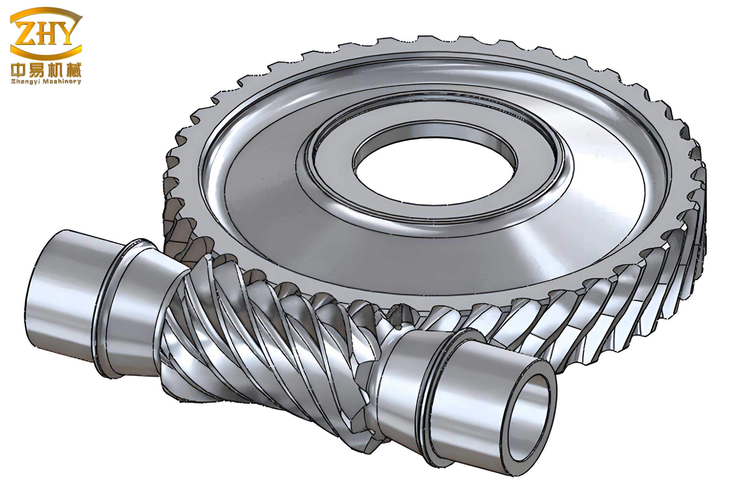
The image above illustrates a typical screw gear system, highlighting the meshing between the worm and worm wheel. Such visual aids are useful for understanding the geometry involved in our optimization model.
To validate the reliability optimization design, we compare it with a conventional design approach. In conventional design, parameters are often selected based on handbooks or empirical rules, with safety factors applied to stresses. For the same application, a conventional design might yield \(Z_1 = 2\), \(q = 10\), and \(m = 6 \text{ mm}\), resulting in a volume of \(2.2631 \times 10^6 \text{ mm}^3\). The table below summarizes the comparison:
| Parameter | Conventional Design | Reliability Optimization Design |
|---|---|---|
| Worm threads, \(Z_1\) | 2 | 2 |
| Diameter factor, \(q\) | 10 | 9 |
| Module, \(m\) (mm) | 6 | 5 |
| Total volume (mm³) | 2.2631 × 10⁶ | 1.34 × 10⁶ |
The optimization reduces the volume by about 40.8%, demonstrating substantial material savings. More importantly, we assess the reliability over time. Using the reliability coefficients derived earlier, we compute the actual reliability for both designs as a function of service years. The life factor \(Z_N\) changes with time because the number of cycles increases. For contact fatigue, \(Z_N = \sqrt[8]{10^7 / N}\), where \(N = 60 n_2 t\), with \(t\) in hours. Assuming 8 hours per day and 300 days per year, we calculate \(Z_N\) for each year and then find \(Z_{R_H}\) and the corresponding reliability \(R_H\) from the normal distribution. The table below shows the reliability for contact fatigue over 10 years for both designs:
| Year | Life Factor, \(Z_N\) | Conventional Design: \(Z_{R_H}\) / \(R_H\) | Optimization Design: \(Z_{R_H}\) / \(R_H\) |
|---|---|---|---|
| 1 | 1.3581 | 6.12 / >0.999999 | 4.05 / 0.999974 |
| 3 | 1.1838 | 5.25 / 0.999999 | 3.18 / 0.999293 |
| 5 | 1.1106 | 4.84 / 0.999999 | 2.77 / 0.997193 |
| 7 | 1.0649 | 4.57 / 0.999995 | 2.50 / 0.993790 |
| 8 | 1.0472 | 4.47 / 0.999992 | 2.40 / 0.991802 |
| 9 | 1.0319 | 4.37 / 0.999987 | 2.30 / 0.989276 |
| 10 | 1.0184 | 4.29 / 0.999980 | 2.22 / 0.986792 |
Note: The reliability values are approximate; for example, \(Z_{R_H} = 4.05\) corresponds to a reliability very close to 1, but we list it as 0.999974 for clarity. In the optimization design, the reliability remains above 0.99 for 8 years, meeting the requirement, whereas the conventional design has excessively high reliability, indicating over-design. This illustrates the efficiency of our approach: it achieves the target reliability precisely, avoiding unnecessary material use while ensuring safety.
For bending fatigue, a similar analysis can be performed. The reliability coefficients \(Z_{R_F}\) are computed, and the results show that the optimization design also satisfies the bending reliability constraint over the intended lifespan. The stiffness constraint is checked numerically; for the optimal parameters, the worm deflection is well below 0.01m, confirming that misalignment risks are mitigated.
The use of MATLAB’s Optimization Toolbox proves effective for solving such nonlinear problems. The fmincon function handles the constraints efficiently, and the SQP algorithm converges to a global optimum for well-behaved functions. In our implementation, we define the objective function and constraints as anonymous functions or separate files, set lower and upper bounds for the variables, and provide initial guesses (e.g., \(Z_1 = 2.5\), \(q = 10\), \(m = 5\)). The solver iterates to find the minimum volume while satisfying all constraints. The ability to incorporate probabilistic reliability into the constraints is a key advantage, as it moves beyond deterministic safety factors.
In broader terms, the reliability optimization design methodology for screw gear systems offers several benefits. First, it provides a systematic way to balance competing objectives: minimizing size or weight while ensuring a specified reliability level. This is crucial in industries like aerospace or automotive, where every gram counts. Second, it accounts for uncertainties in loads, materials, and manufacturing, leading to more robust designs. Third, the mathematical framework is generalizable; with adjustments, it can be applied to other gear types, such as helical gears or bevel gears, or to different failure modes like thermal failure in screw gear systems due to friction-induced heating. Future work could explore multi-objective optimization, where both volume and cost are minimized, or include dynamic effects like vibration and noise. Additionally, advanced probability distributions, such as Weibull for fatigue life, could be integrated for more accurate reliability modeling.
In conclusion, we have presented a comprehensive approach to reliability optimization design for screw gear transmission systems. By combining log-normal stress-strength interference models with nonlinear programming, we derived optimal parameters that minimize volume subject to reliability constraints. The case study demonstrates that this method yields significant material savings—over 40% volume reduction—compared to conventional design, while still meeting a 0.99 reliability requirement over an 8-year service life. The integration of MATLAB tools streamlines the solution process, making it accessible for engineers. This work underscores the importance of merging reliability and optimization theories in mechanical design, particularly for critical components like screw gears. As technology advances, such methodologies will become increasingly vital for developing efficient, safe, and cost-effective mechanical systems. We hope this article inspires further research and application in the field, extending the principles to other complex mechanical assemblies.