
In the realm of mechanical transmission systems, screw gears, particularly double lead screw gears, hold a pivotal role due to their ability to achieve high-precision motion control and backlash adjustment. As an engineer engaged in the design and analysis of gear systems, I have often encountered challenges in creating accurate three-dimensional models for such components. Traditional modeling approaches frequently fall short in capturing the intricate geometry of screw gears, especially when dealing with non-standard tooth profiles or varying lead parameters. This article presents a comprehensive, first-person account of a precise modeling method for double lead screw gears using UG software, grounded in the fundamental working and manufacturing principles of these gears. Our method leverages the concept of tool-workpiece contact lines undergoing helical motion to generate exact tooth surfaces, which are then used to derive conjugate gear profiles. Throughout this discussion, we will emphasize the term “screw gears” to underscore their helical nature and widespread applicability.
Double lead screw gears operate on the same basic principle as standard cylindrical worm gears but with a distinctive feature: the left and right tooth flanks possess different leads, while the lead on each flank remains constant. This design results in a progressive variation in axial tooth thickness along the gear’s length. The primary advantage lies in the ability to adjust meshing backlash by axially shifting the screw gear, thereby maintaining optimal contact without altering the center distance—a common drawback in radial adjustment methods. In essence, the double lead screw gear functions as a variable-thickness齿条 in the axial plane, engaging with a gear that has uniform tooth thickness. This characteristic makes double lead screw gears indispensable in precision applications such as indexing tables, rotary actuators, and high-accuracy reducers where minimal play is critical.
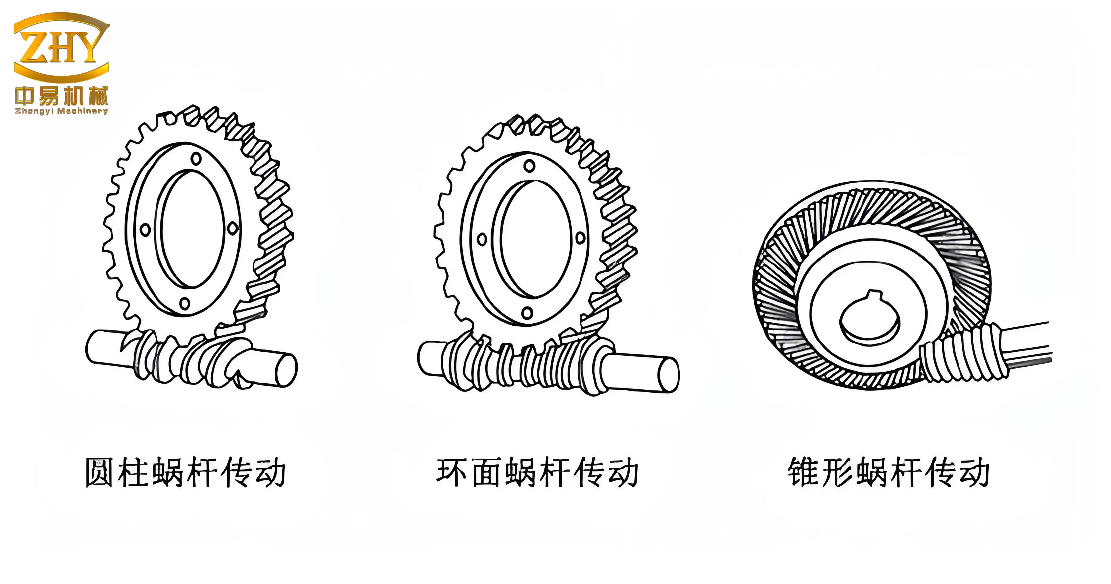
The manufacturing process for screw gears typically involves turning with straight-edged cutting tools. The orientation of the tool relative to the workpiece determines the type of helical surface generated. For instance, when the tool edge lies in the axial plane of the screw gear, an Archimedean spiral surface is produced; when placed in the normal plane, an extended involute surface results; and when positioned tangent to the base cylinder, a true involute helicoid is formed. This turning operation can be conceptualized as the contact line between the tool and the screw gear blank undergoing a simultaneous rotation and translation—a helical motion. By accurately defining this motion for each tooth flank, we can derive the precise mathematical representation of the screw gear’s tooth surface. This understanding forms the bedrock of our modeling strategy, which aims to replicate the actual machining process within UG to achieve geometrically faithful models.
To mathematically describe the tooth surface of a screw gear, we employ vector algebra. Consider a position vector $\mathbf{r}(x, y, z)$ in a coordinate system $O-ijk$. When this vector rotates around the $k$-axis by an angle $\phi_k$, the transformed coordinates are given by:
$$
\begin{bmatrix} x’ \\ y’ \\ z’ \end{bmatrix} = \begin{bmatrix} \cos \phi_k & -\sin \phi_k & 0 \\ \sin \phi_k & \cos \phi_k & 0 \\ 0 & 0 & 1 \end{bmatrix} \begin{bmatrix} x \\ y \\ z \end{bmatrix}
$$
Similarly, rotation about the $j$-axis or $i$-axis yields corresponding transformation matrices. Now, if the vector simultaneously undergoes a linear displacement along the $k$-axis proportional to the rotation angle, we obtain a helical motion. Let $p$ be the helical parameter (lead per radian, where $p > 0$ for right-hand helices and $p < 0$ for left-hand helices). The combined transformation is:
$$
\begin{bmatrix} x’ \\ y’ \\ z’ \end{bmatrix} = \begin{bmatrix} \cos \phi_k & -\sin \phi_k & 0 \\ \sin \phi_k & \cos \phi_k & 0 \\ 0 & 0 & 1 \end{bmatrix} \begin{bmatrix} x \\ y \\ z \end{bmatrix} + \begin{bmatrix} 0 \\ 0 \\ p \phi_k \end{bmatrix}
$$
If we consider $\mathbf{r}(t) = [x(t), y(t), z(t)]^T$ as a parameterized curve representing the tool’s cutting edge (i.e., the contact line), then as the parameter $t$ and rotation angle $\phi_k$ vary, the equation above generates a helical surface—the tooth flank of the screw gear. For a double lead screw gear, we have two distinct helical parameters: $p_L$ for the left flank and $p_R$ for the right flank, corresponding to their respective leads. Thus, the left and right tooth surfaces are defined separately by:
$$
\mathbf{r}_L'(t, \phi) = \mathbf{R}_z(\phi) \cdot \mathbf{r}_L(t) + [0, 0, p_L \phi]^T, \quad \mathbf{r}_R'(t, \phi) = \mathbf{R}_z(\phi) \cdot \mathbf{r}_R(t) + [0, 0, p_R \phi]^T
$$
where $\mathbf{R}_z(\phi)$ is the rotation matrix about the z-axis. This formulation allows us to model any type of screw gear—Archimedean, extended involute, or involute—by appropriately defining the initial tool edge curve $\mathbf{r}(t)$. The key is to determine the endpoints of these contact lines based on the gear’s dimensional parameters and then generate their helical trajectories.
Let us illustrate the parameter computation with a concrete example of an extended involute double lead screw gear, commonly used in precision rotary tables. The following table summarizes the basic design parameters for both the screw gear and the mating gear:
| Parameter Description | Symbol | Value | Unit |
|---|---|---|---|
| Nominal axial module | $m$ | 1.5 | mm |
| Number of threads on screw gear | $z_1$ | 1 | – |
| Number of teeth on gear | $z_2$ | 80 | – |
| Normal pressure angle | $\alpha_{on}$ | 15° | degree |
| Left flank axial pitch | $t_z$ | 4.7686 | mm |
| Right flank axial pitch | $t_y$ | 4.6561 | mm |
| Screw gear pitch diameter | $d_{f1}$ | 32 | mm |
| Center distance | $A$ | 76 | mm |
| Addendum coefficient | $f_0$ | 1 | – |
| Dedendum coefficient | $c_0$ | 0.2 | – |
From these, we derive the essential geometric parameters. The nominal axial pitch is $t_0 = m\pi = 4.7124 \text{ mm}$. The pitch difference is $\Delta t = (t_z – t_y)/2 = 0.0563 \text{ mm}$. The left and right flank modules are $m_z = t_z/\pi = 1.5179 \text{ mm}$ and $m_y = t_y/\pi = 1.4821 \text{ mm}$, respectively. The module deviation from nominal is $\Delta m = m_z – m = m – m_y = 0.0179 \text{ mm}$. The thickness increment coefficient is $k_s = (t_z – t_y)/t_0 = 0.02387$.
For the screw gear, the effective pitch diameters for left and right flanks, considering profile shift due to double lead, are:
$$
d_{1z} = d_{f1} – \Delta m \cdot z_2 = 30.568 \text{ mm}, \quad d_{1y} = d_{f1} + \Delta m \cdot z_2 = 33.432 \text{ mm}
$$
The corresponding lead angles on these pitch cylinders are:
$$
\lambda_z = \arctan\left( \frac{m_z z_1}{d_{1z}} \right) = 2.8428^\circ, \quad \lambda_y = \arctan\left( \frac{m_y z_1}{d_{1y}} \right) = 2.5384^\circ
$$
Since the gear is of extended involute type with a normal pressure angle, the axial pressure angles for each flank are computed as:
$$
\alpha_{oaz} = \arctan\left( \frac{\tan \alpha_{on}}{\cos \lambda_z} \right) = 15.0134^\circ, \quad \alpha_{oay} = \arctan\left( \frac{\tan \alpha_{on}}{\cos \lambda_y} \right) = 15.0117^\circ
$$
For the mating gear, the nominal pitch diameter is $d_{f2} = m z_2 = 120 \text{ mm}$, with addendum diameter $d_{e2} = m(z_2 + 2f_0) = 123 \text{ mm}$. The effective pitch diameters for left and right flanks are $d_{f2z} = m_z z_2 = 121.432 \text{ mm}$ and $d_{f2y} = m_y z_2 = 118.568 \text{ mm}$, respectively. Their base circle diameters are $d_{oz} = d_{f2z} \cos \alpha_{oaz} = 117.2912 \text{ mm}$ and $d_{oy} = d_{f2y} \cos \alpha_{oay} = 114.5248 \text{ mm}$.
An important aspect in designing screw gears is determining the necessary helical length $L$ to ensure proper engagement without excess material. This length comprises the active contact length $L_\alpha$, a process length $L_t$ for manufacturing, and an adjustment length $L_p$ for backlash control. Through geometric analysis of the meshing lines, we calculate:
$$
L_\alpha = \max(e_{y2}, e_{z1}) + \max(e_{y1}, e_{z2}) \approx 11.9909 \text{ mm}, \quad L_t = 2m\pi = 9.4248 \text{ mm}, \quad L_p = \frac{\Delta s}{k_s} \approx 9.0907 \text{ mm}
$$
where $\Delta s = 0.2 \text{ mm}$ is the desired adjustment range, and $e$ terms are engagement segment lengths derived from tooth geometry. Thus, total length $L = L_\alpha + L_t + L_p \approx 30.5064 \text{ mm}$. Additionally, the minimum axial tooth tip width $S_a$ and root width $b_{min}$ are checked to avoid weak sections:
$$
S_a = \frac{1}{2}\pi m – \frac{1}{2} L k_s – f_0 m (\tan \alpha_{oaz} + \tan \alpha_{oay}) \approx 1.1875 \text{ mm}, \quad b_{min} = \frac{1}{2}\pi m (1 + k_s) – \frac{1}{2} L k_s – (f_0 + c_0) m (\tan \alpha_{oaz} + \tan \alpha_{oay}) \approx 1.0816 \text{ mm}
$$
With parameters fully defined, we proceed to the UG modeling phase. Our goal is to create the double lead screw gear by simulating the helical motion of the tool contact lines. We start by establishing a coordinate system with the Z-axis along the screw gear’s axis and the X-axis through the center of a reference tooth space at the thin-end side. The endpoints of the left and right tool edges (contact lines) in the axial cross-section are identified. For the extended involute case, these are points A, B, C, D with coordinates (in mm): A(17.5, -1.9031), B(14.2, -1.018), C(17.5, 1.903), D(14.2, 1.0181) in the X-Z plane (Y=0).
In UG NX10, we use the “Expression” tool under “Tools” to define variables for leads, angles, and coordinates. The left and right helical parameters are $p_L = t_z / (2\pi)$ and $p_R = t_y / (2\pi)$ for the respective leads. Using the “Law Curve” function under “Insert > Curve”, we input parametric equations based on the helical motion formula to generate four helical curves corresponding to the trajectories of points A, B, C, D. For point A on the left flank, the equations are:
$$
x = X_1 \cos(\phi) – Y_1 \sin(\phi), \quad y = X_1 \sin(\phi) + Y_1 \cos(\phi), \quad z = Z_1 + p_L \phi
$$
with $\phi$ varying over a sufficient range to cover the helical length $L$. Similar expressions are set for other points. This yields two pairs of helical curves defining the boundaries of the left and right tooth spaces.
Once the helical curves are generated, we use surface modeling commands to create the tooth flanks. The “Ruled Surface” or “Through Curve Mesh” functions under “Insert > Mesh Surface” are employed to create surfaces between corresponding helical curves. For instance, the surface between the helices of A and B forms part of the left flank, while that between C and D forms part of the right flank. The “Bounded Surface” command can fill the ends. All surfaces are then stitched together using “Sew” under “Insert > Combine” to form a solid tooth space. This solid represents the void where material will be removed.
Next, we create the screw gear blank as a cylinder with diameter equal to the addendum diameter and length exceeding $L$. Using “Subtract” Boolean operation, we remove the tooth space solid from the blank, resulting in a single helical tooth. To complete the screw gear, we apply a circular pattern around the axis, with the number of instances equal to the virtual number of teeth over the active length. Since the tooth thickness varies axially, the pattern must account for the progressive phase shift. In UG, this can be achieved by defining a pattern along a helix or by incremental rotation and translation. The outcome is a precise three-dimensional model of the double lead screw gear, accurately reflecting the varying lead and tooth profile.
Modeling the mating gear (the wheel) leverages the conjugate action principle. In an assembly context, we use the “WAVE Geometry Linker” in UG to copy the screw gear’s tooth surface as a reference onto the gear blank. Then, via Boolean subtraction, we generate the gear tooth spaces. However, due to the double lead, the initial subtracted cavity may be irregular. We refine this by extracting boundary curves from a representative tooth space cross-section using “Insert > Derived Curve > Extract”. These curves are used to construct a clean, filled surface, which is then stitched into a solid. This solid tooth space is patterned circularly with 80 instances (matching $z_2$) and subtracted from the gear blank, yielding the final gear model. This approach ensures accurate tooth geometry derived directly from the screw gear’s active profiles.
The presented methodology offers several advantages. First, it is universally applicable to various types of screw gears—Archimedean, extended involute, or involute—simply by adjusting the initial tool edge coordinates. Second, it faithfully replicates the actual manufacturing process, leading to geometrically exact models. Third, the use of UG’s parametric and associative design features allows for easy modifications; changing a parameter like lead or module updates the entire model automatically. This is particularly beneficial for iterative design and analysis. Fourth, the models serve as reliable inputs for subsequent engineering simulations, such as finite element analysis for stress evaluation, kinematic studies for motion accuracy, or CNC programming for direct manufacturing.
To further illustrate the parameter relationships and computational steps, we consolidate key formulas in the following table, which can serve as a quick reference for designers working with double lead screw gears:
| Calculation | Formula | Notes |
|---|---|---|
| Left/Right Module | $m_{z,y} = t_{z,y} / \pi$ | From axial pitches |
| Lead Angle per Flank | $\lambda_{z,y} = \arctan( m_{z,y} z_1 / d_{1z,1y} )$ | On effective pitch diameter |
| Axial Pressure Angle | $\alpha_{oa z,y} = \arctan( \tan \alpha_{on} / \cos \lambda_{z,y} )$ | For normal pressure angle $\alpha_{on}$ |
| Helical Surface Generation | $\mathbf{r}’ = \mathbf{R}_z(\phi) \mathbf{r}(t) + [0,0, p \phi]^T$ | $p$: lead parameter, $\mathbf{r}(t)$: tool edge |
| Active Length Component | $L_\alpha = \max(e_1, e_2) + \max(e_3, e_4)$ | Based on engagement geometry |
| Tooth Thickness Variation | $\Delta S = k_s \cdot \text{axial position}$ | $k_s$: thickness increment coefficient |
In conclusion, the precision modeling of double lead screw gears using UG software, as detailed from a first-person perspective, provides a robust and accurate approach to capturing their complex geometry. By grounding the method in the physical machining process—where tool contact lines undergo defined helical motions—we ensure that the resulting digital models are true to life. This methodology not only simplifies the modeling of screw gears with varying leads and tooth profiles but also enhances the reliability of downstream engineering analyses. As screw gears continue to be critical in high-precision mechanical systems, such precise modeling techniques become indispensable for design validation, performance optimization, and manufacturing preparation. The integration of parametric design, advanced surface modeling, and conjugate gear generation within UG establishes a comprehensive framework for handling the intricacies of double lead screw gears, ultimately contributing to more efficient and accurate mechanical transmissions.